Transmitted Flux Power Spectrum
The input to the Flux Power Spectrum is then flux as function of velocity, i.e. F (v), over some velocity interval \(V\) (in the data set this interval is chosen so that one avoids the Lyman-\(\beta\) forest, the quasar near zone, and potentially some strong absorbers; in the simulations it is set by the linear extent of the simulated volume).
Given F and its mean, \(\langle F \rangle\), we calculate the ‘normalized flux’
\[\delta_{F} \equiv \frac{F-\langle F\rangle}{\langle F\rangle}\]The FPS is written in terms of the dimensionless variance \(\Delta_F^2(k)\) (strictly speaking a variance in \(\delta_F\) per dex in \(k\)), defined by
\[\Delta_{F}^{2}(k)=\frac{1}{\pi} k P_{F}(k)\] \[P_{F}(k)=V \bigg \langle \left|\tilde{\delta}_{F}(k)\right|^{2} \bigg \rangle\] \[\tilde{\delta}_{F}(k)=\frac{1}{V} \int_{0}^{V} d v e^{-i k v} \delta_{F}(v)\]Here, \(\langle \cdot \rangle\) denotes the ensemble average, and \(k = 2\pi/v\) is the Fourier ‘frequency’ corresponding to \(v\) and has dimensions of (s/km).
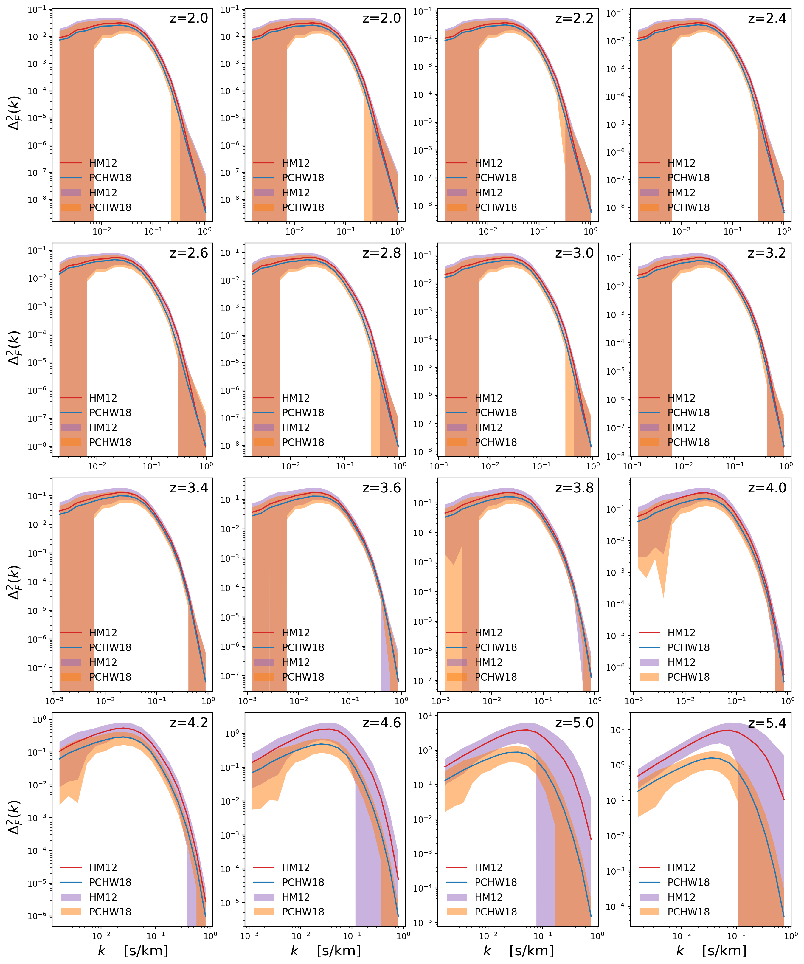
Power Spectrum for several redshifts
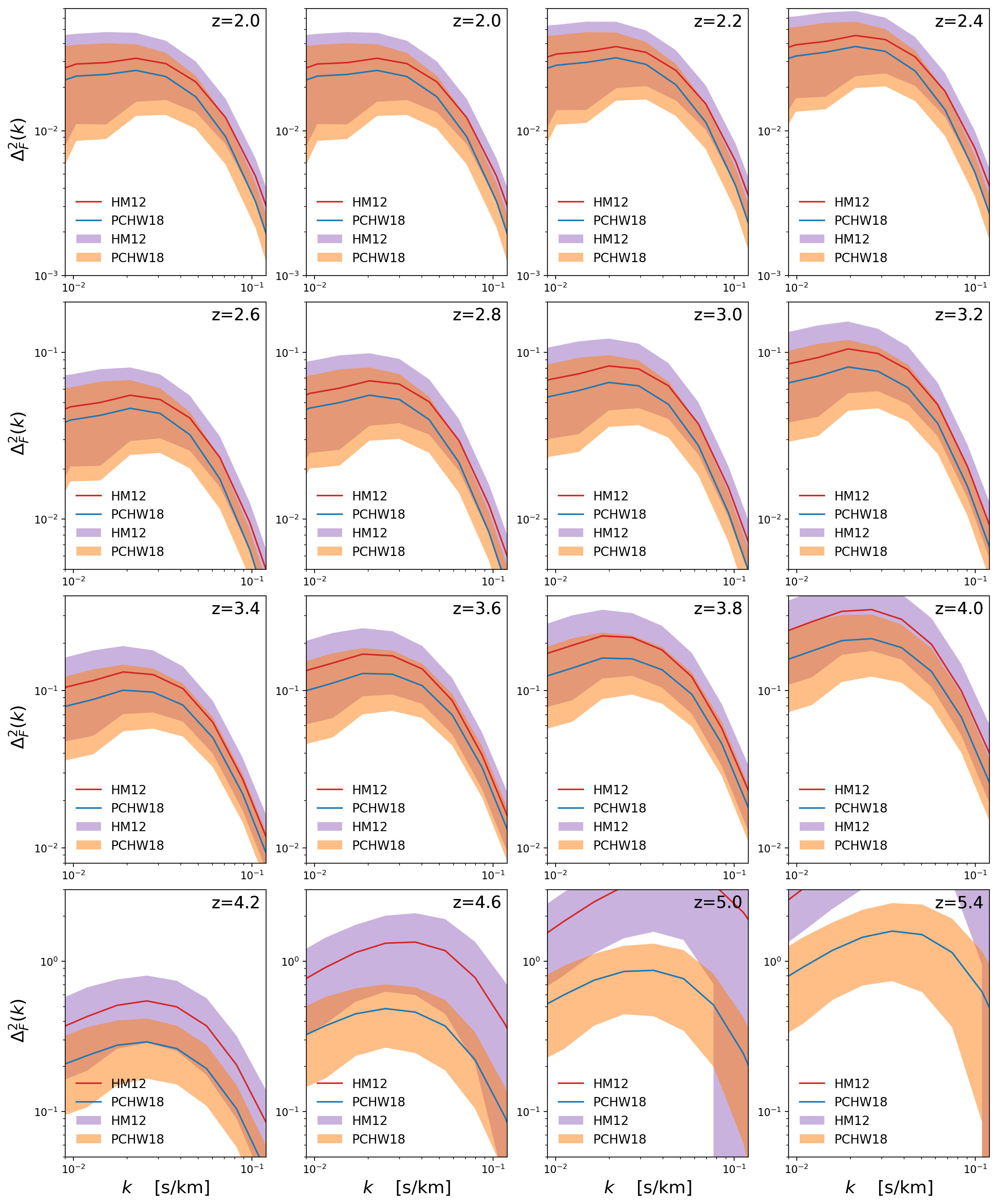
Now limiting the range in \(k\)
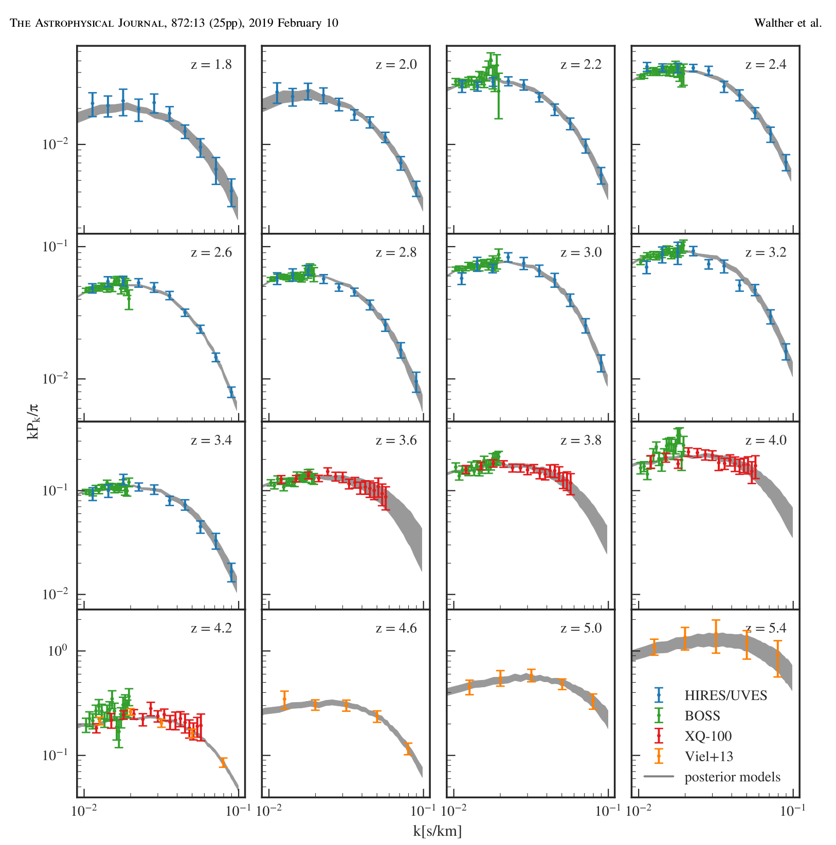
Compared to results from Walther+2019