SPH Kernel Density
From the Gadget2 paper:
The kernel as a function of distance \(r\) and smoothing length \(h\) is given by:
\[W(r, h)=\frac{8}{\pi h^{3}}\left\{\begin{array}{ll} 1-6\left(\frac{r}{h}\right)^{2}+6\left(\frac{r}{h}\right)^{3}, & 0 \leqslant \frac{r}{h} \leqslant \frac{1}{2} \\ 2\left(1-\frac{r}{h}\right)^{3}, & \frac{1}{2}<\frac{r}{h} \leqslant 1 \\ 0, & \frac{r}{h}>1 \end{array}\right.\]Of fundamental importance for any SPH formulation is the density estimate, which GADGET-2 does in the form \(\rho_{i}=\sum_{j=1}^{N} m_{j} W\left(\left|\boldsymbol{r}_{i j}\right|, h_{i}\right)\)
where \(r_{ij} ≡ r_i − r_j\) , and \(W(r, h)\) is the SPH smoothing kernel defined in equation (4).2 In our ‘entropy formulation’ of SPH, the adaptive smoothing lengths \(h_i\) of each particle are defined such that their kernel volumes contain a constant mass for the estimated density, i.e. the smoothing lengths and the estimated densities obey the (implicit) equations \(\frac{4 \pi}{3} h_{i}^{3} \rho_{i}=N_{\mathrm{sph}} \bar{m}\) where \(N_{\mathrm{sph}}\) is the typical number of smoothing neighbours, and \(\bar{m}\) is an average particle mass.
Some things to notice:
The density at the \(i\) particle position is computed by:
\[\rho_{i}=\sum_{j=1}^{N} m_{j} W\left(\left|\mathbf{r}_{i j}\right|, h_{i}\right)\]note that the smoothing length used is \(h_i\) and not the smoothing length of the neighbors.
Measuring \(N_{\mathrm{sph}}\)
From the equation:
\[\frac{4 \pi}{3} h_{i}^{3} \rho_{i}=N_{\mathrm{sph}} \bar{m}\]I can use the values of \(\rho_i\) and \(h_i\) from the file to compute \(N_{\mathrm{sph}}\), this is the distribution of values that I get.
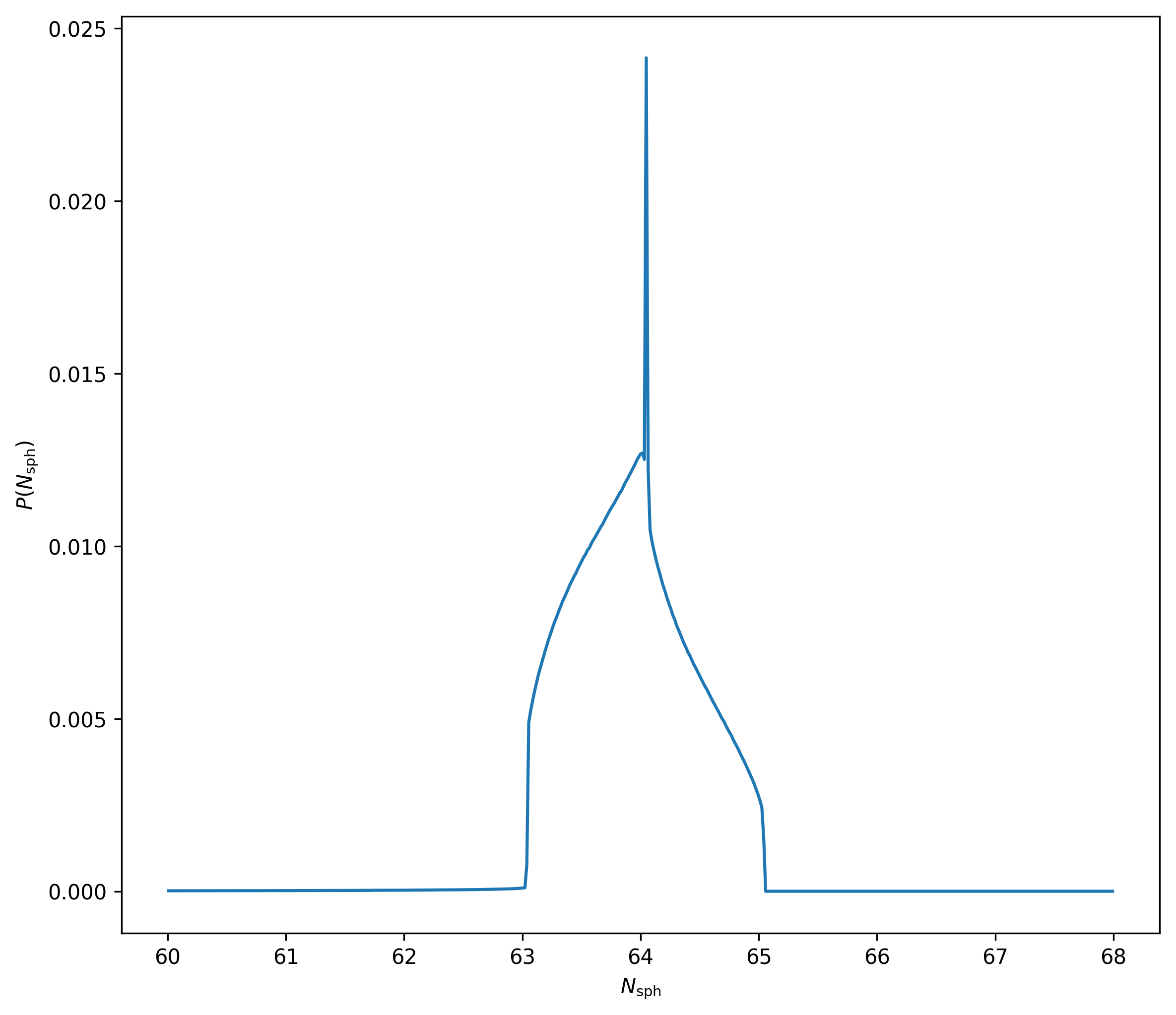
So, it seems like \(N_{\mathrm{sph}} \approx 64\)
Measuring \(N_{\mathrm{neighbors}}\) within \(h_i\)
Now for each particle I measure the number of neighbors \(N_{\mathrm{neighbors}}\) within the smoothing length \(h_i\) obtained from the data file, the distribution is below:
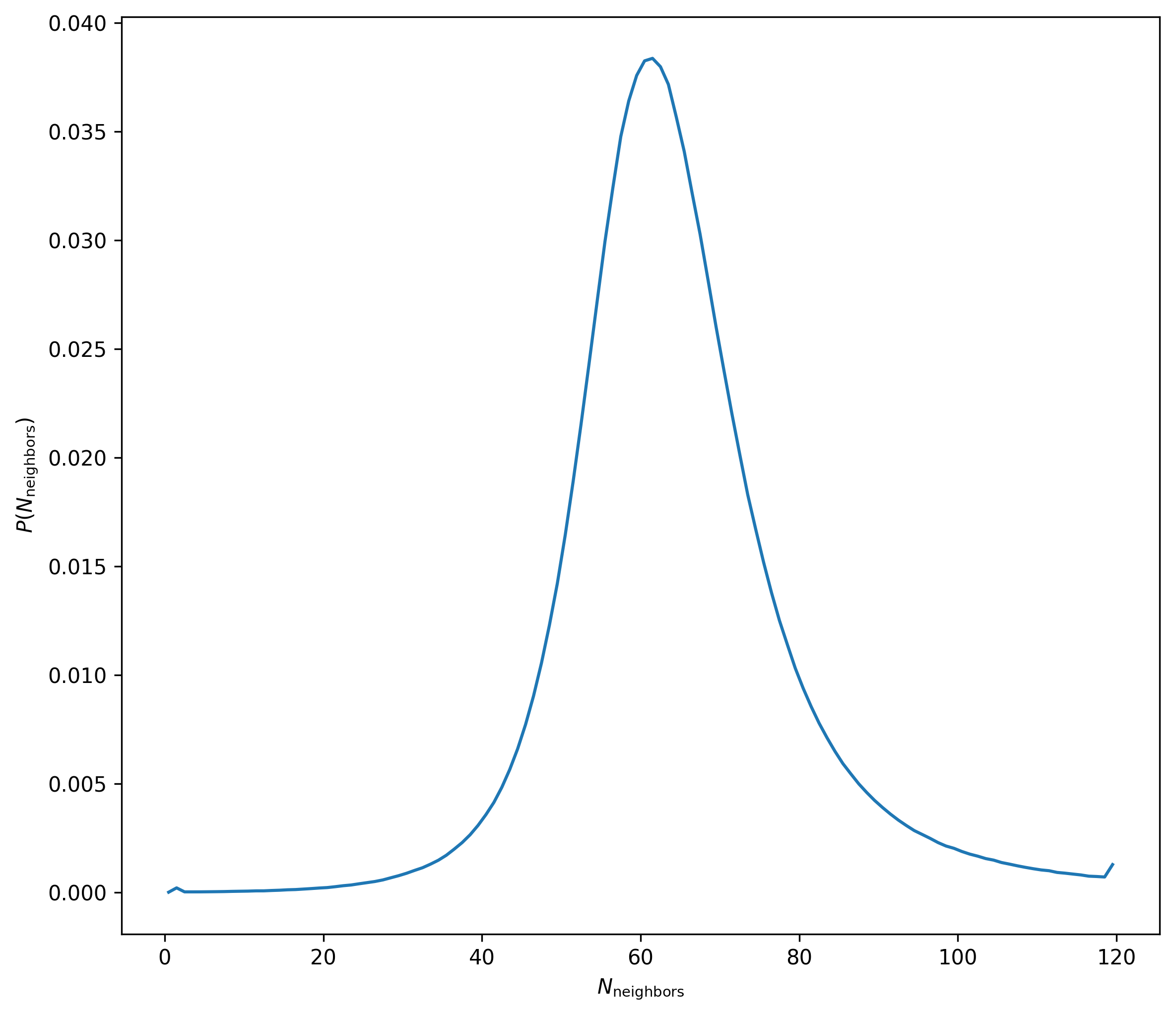
So it’s clear that not all particles have 64 neighboring particles within their smoothing length.
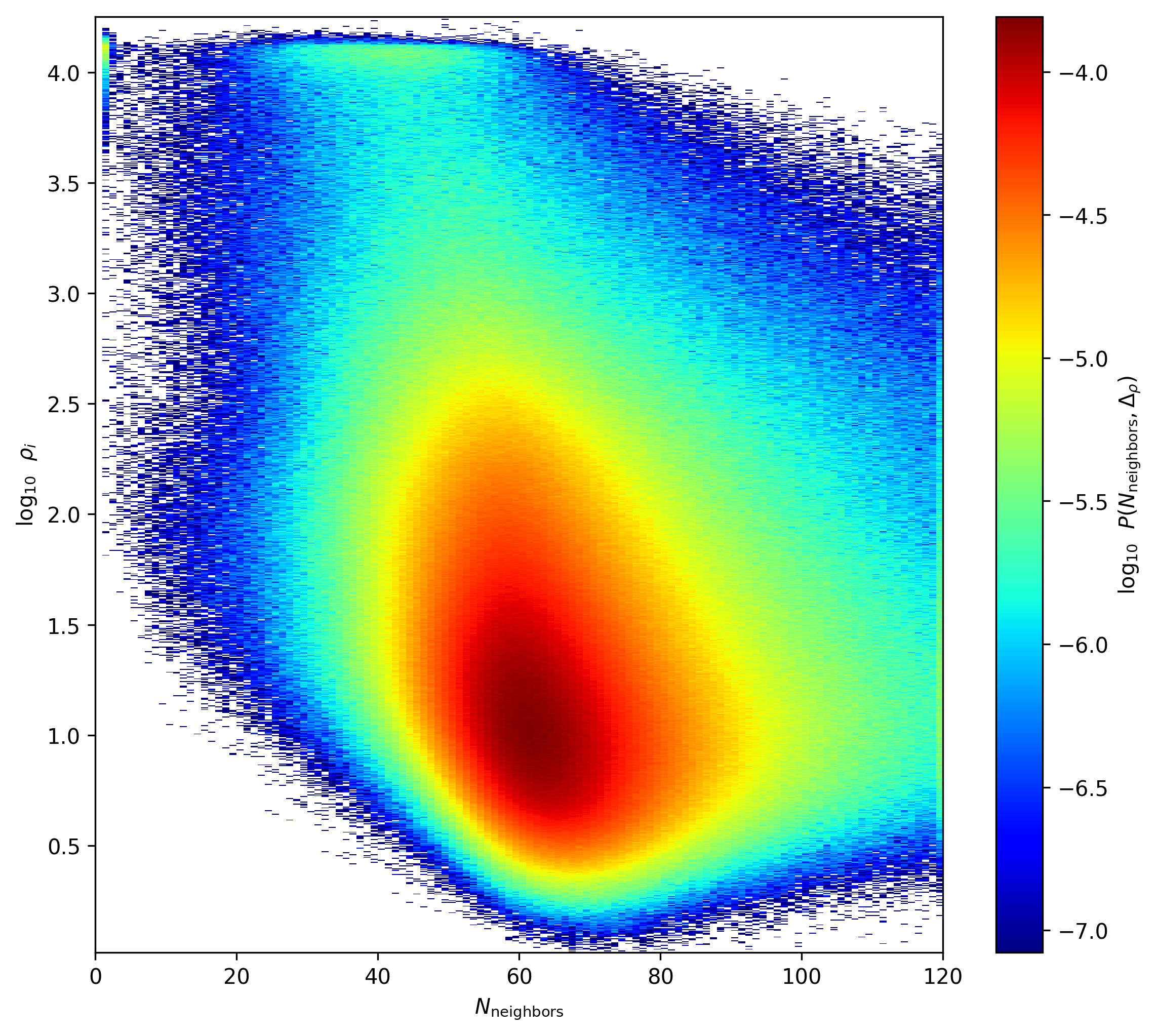
Density and \(N_{\mathrm{neighbors}}\) Distribution
This shows the distribution of \(\rho_i\) in the field against the number of neighbors within \(h_i\) , the number of neighbors includes the central particle so N_neighbors=1 means that there are no other particles within \(h_i\) other than the central particle
Density Comparison Using Gadget \(h_i\)
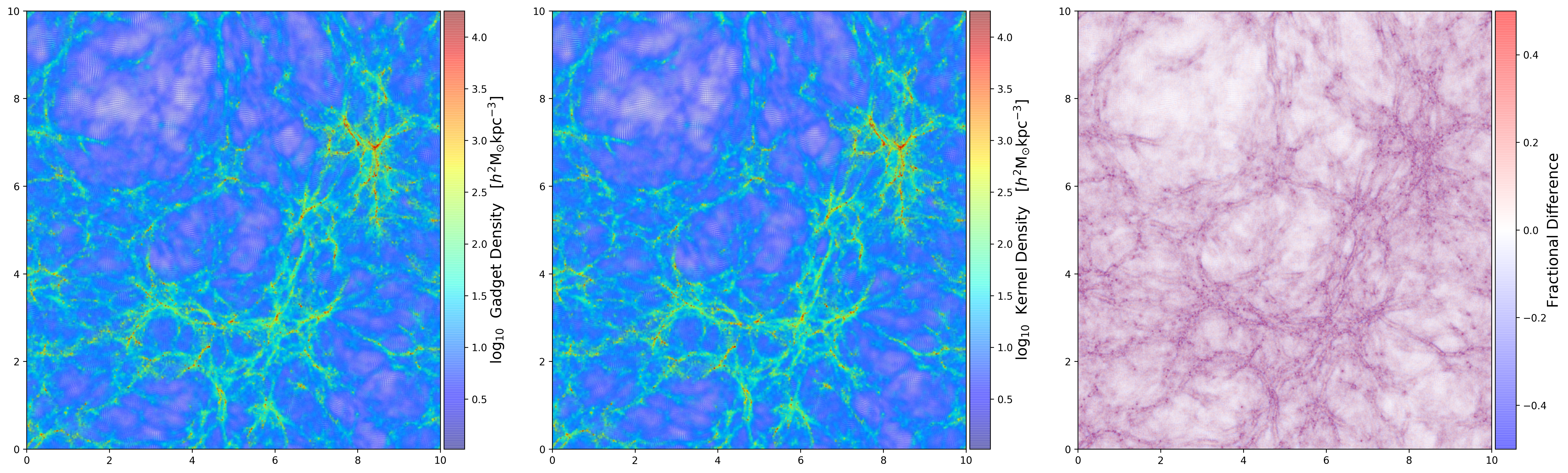
First I compute the density passing the smoothing length \(h_i\) that I get from the data file.
Panel 1: Density on the data file. Panel 2: Density computed from the kernel using \(h_{64}\). Panel 3: Fractional difference between the two densities.
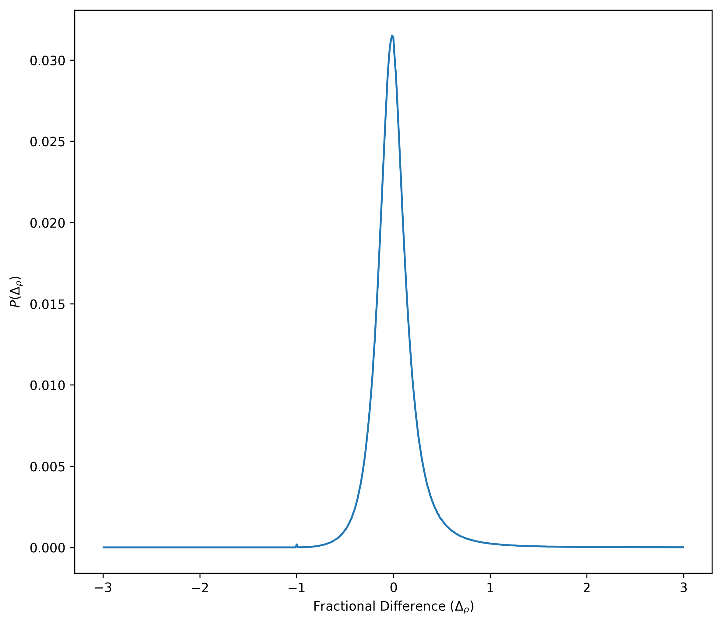
Now I show the distribution of the fractional differences
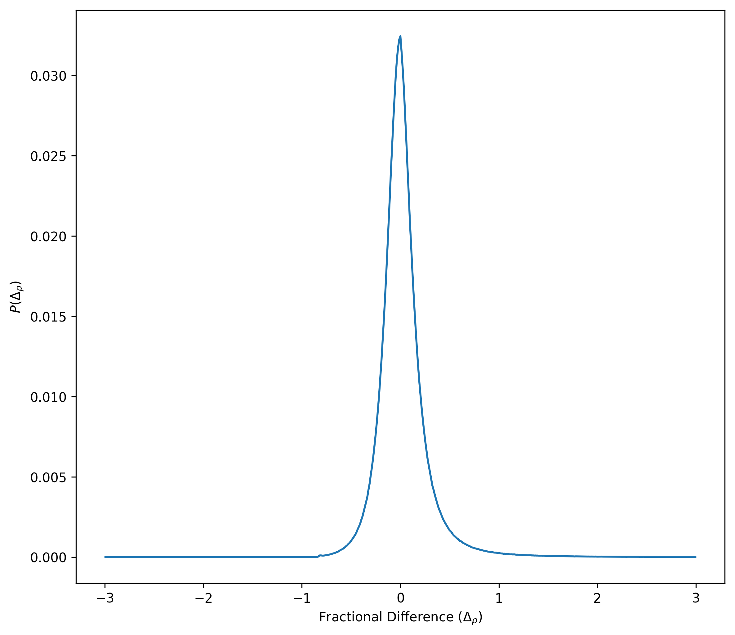
Here is the fractional difference vs. density distribution
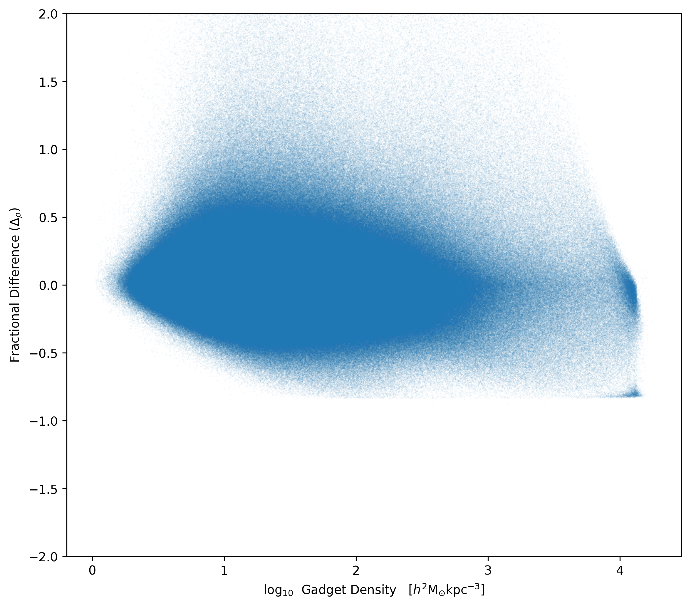
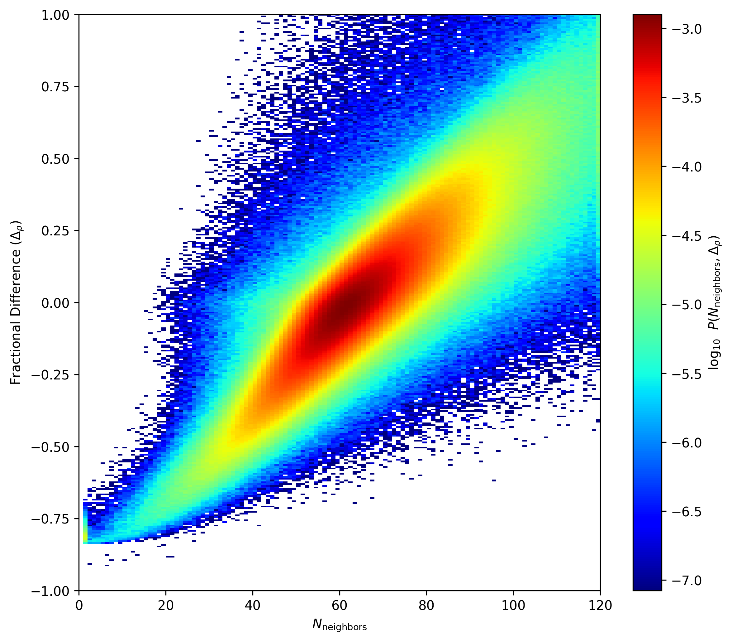
Here is fractional difference vs. N_neighbors difference
Now I focus on the 4000 particles with highest density an measure the fractional difference as I change the number of neighbors to compute the smoothing length.
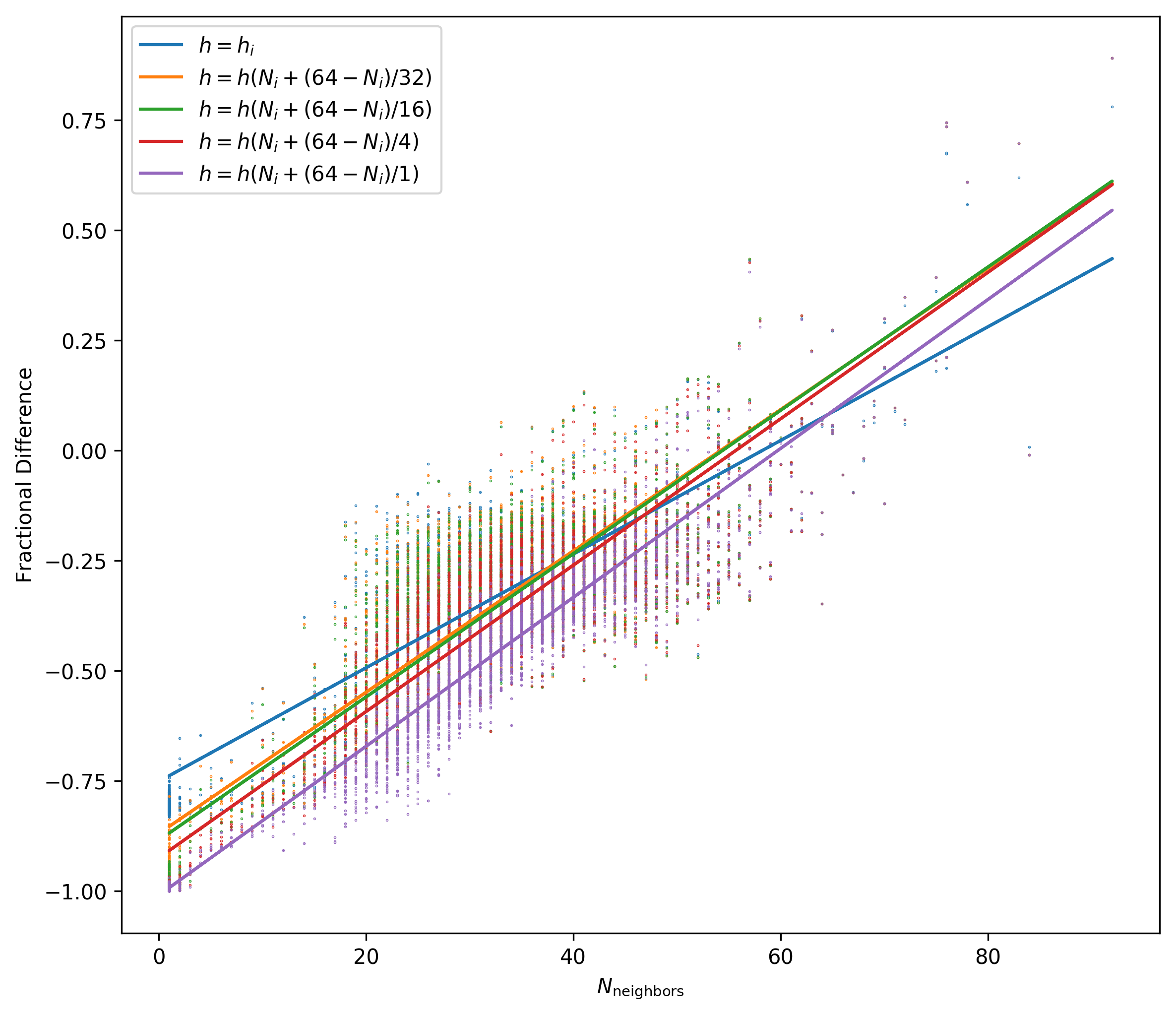
Changing the Number of neighbors to get them closer to 64 just increases the Fractional Difference
Density Comparison Using \(h_{64}\)
Now I compute the density passing the smoothing length \(h_{64}\) which is the radius that encloses 64 neighbors.
Panel 1: Density on the data file. Panel 2: Density computed from the kernel using \(h_i\) from the data file. Panel 3: Fractional difference between the two densities.

Now I show the distribution of the fractional differences
There densities computed with the two different smoothing length are not significantly different.
Density Comparison Using \(h_{64}\) compared to \(h_i\)
This shows the fractional difference between densities computed using \(h_i\) and \(h_{64}\).
\[\Delta_{\rho} = \frac{\rho_{h_{64}} - \rho_{h_{i}}}{\rho_{h_{i}}}\]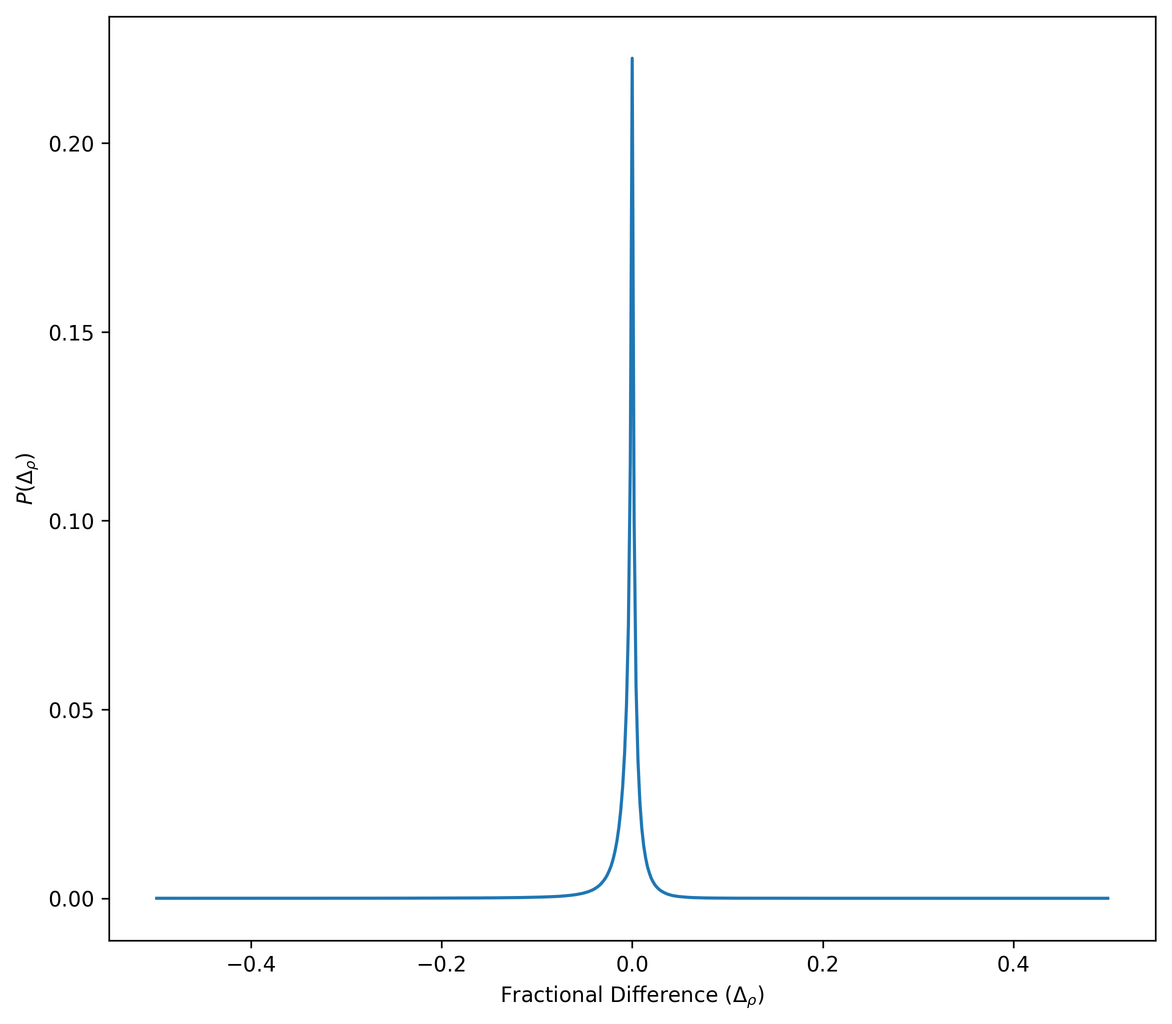
The differences are less than 5%.