WDM MCMC Fitting using covariance matrix
After recomputing the flux power spectrum natively on the same \(k\)-bins as Boera et al. (instead of interpolating) to avoid correlations on adjacent Fourier modes I redo the MCMC fitting.
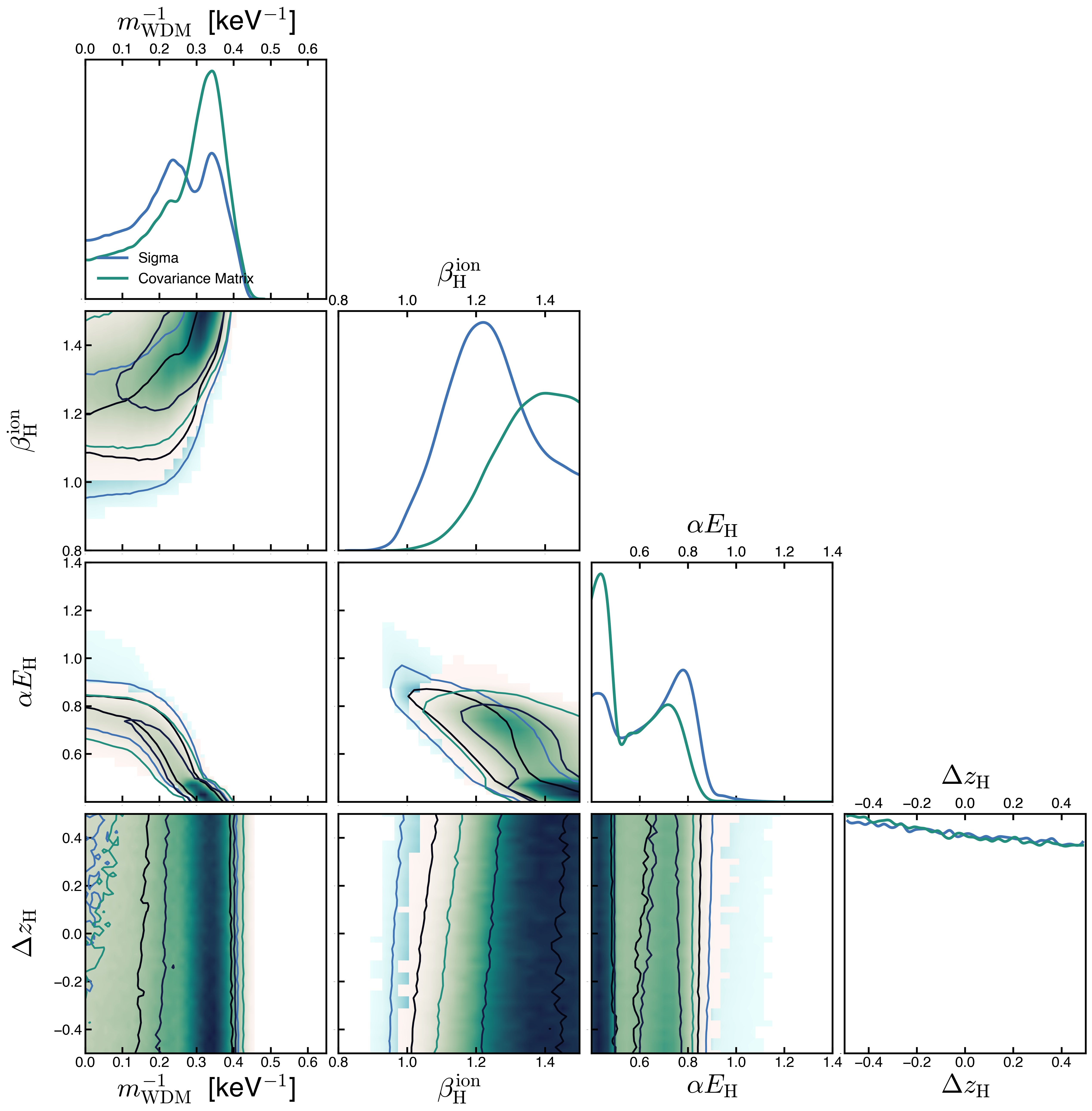
Here I compare the fits that result from using the uncertainty \(sigma\) against using the full covariance matrix from Boera et al. The results are not that different now.
Joint Fit to all redshifts
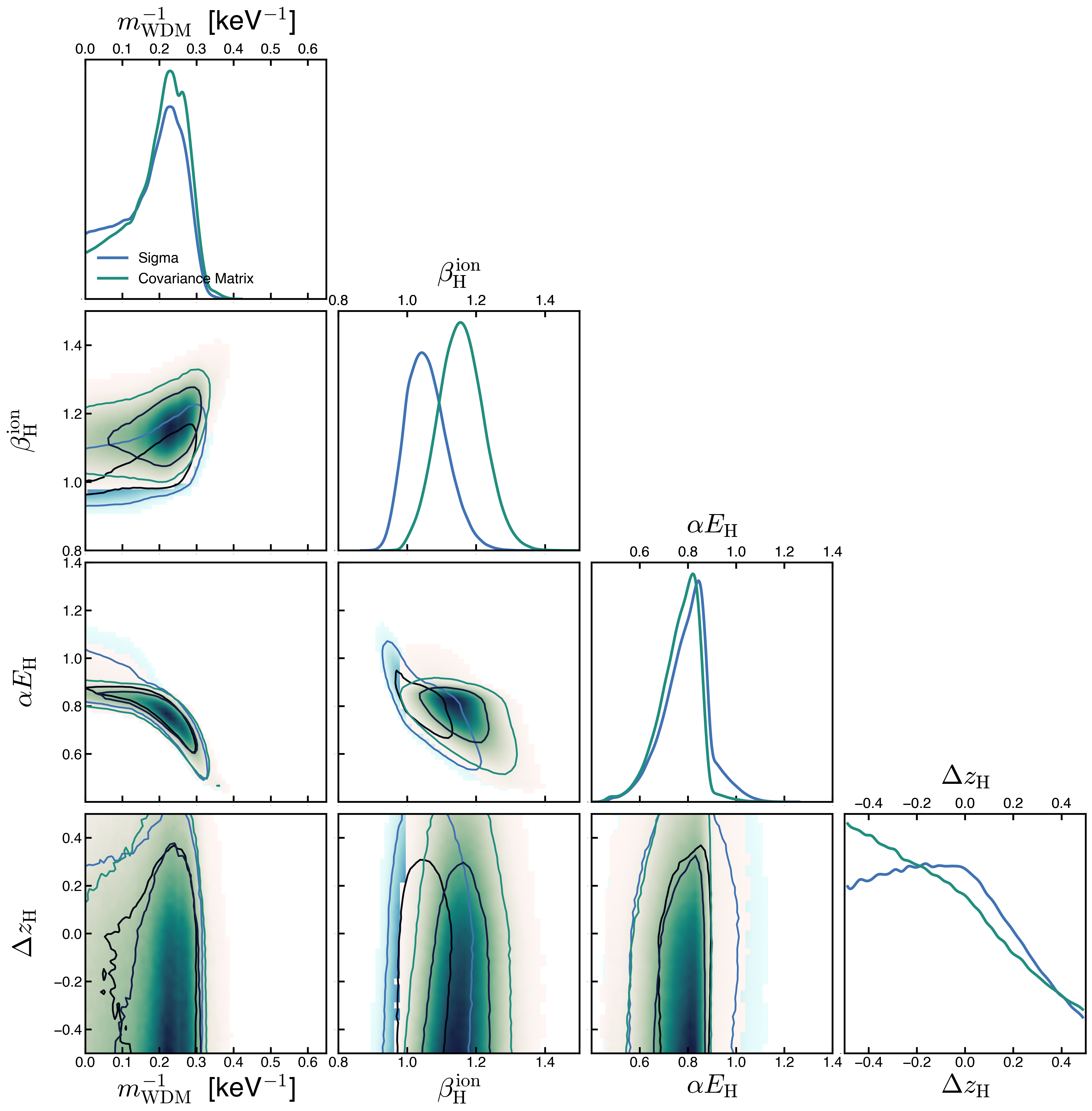
Fit only to \(z=4.2\)
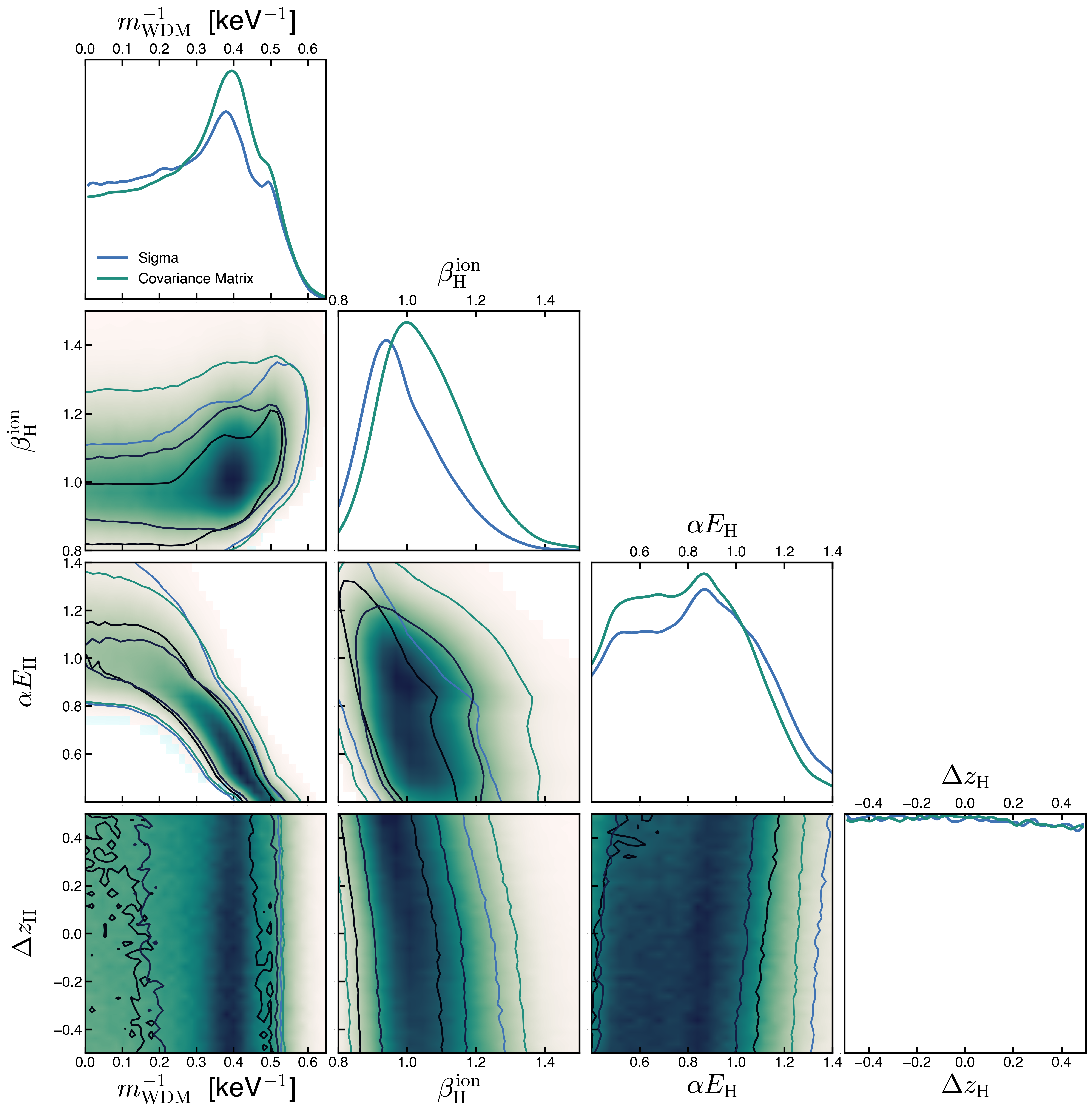
Fit only to \(z=4.6\)
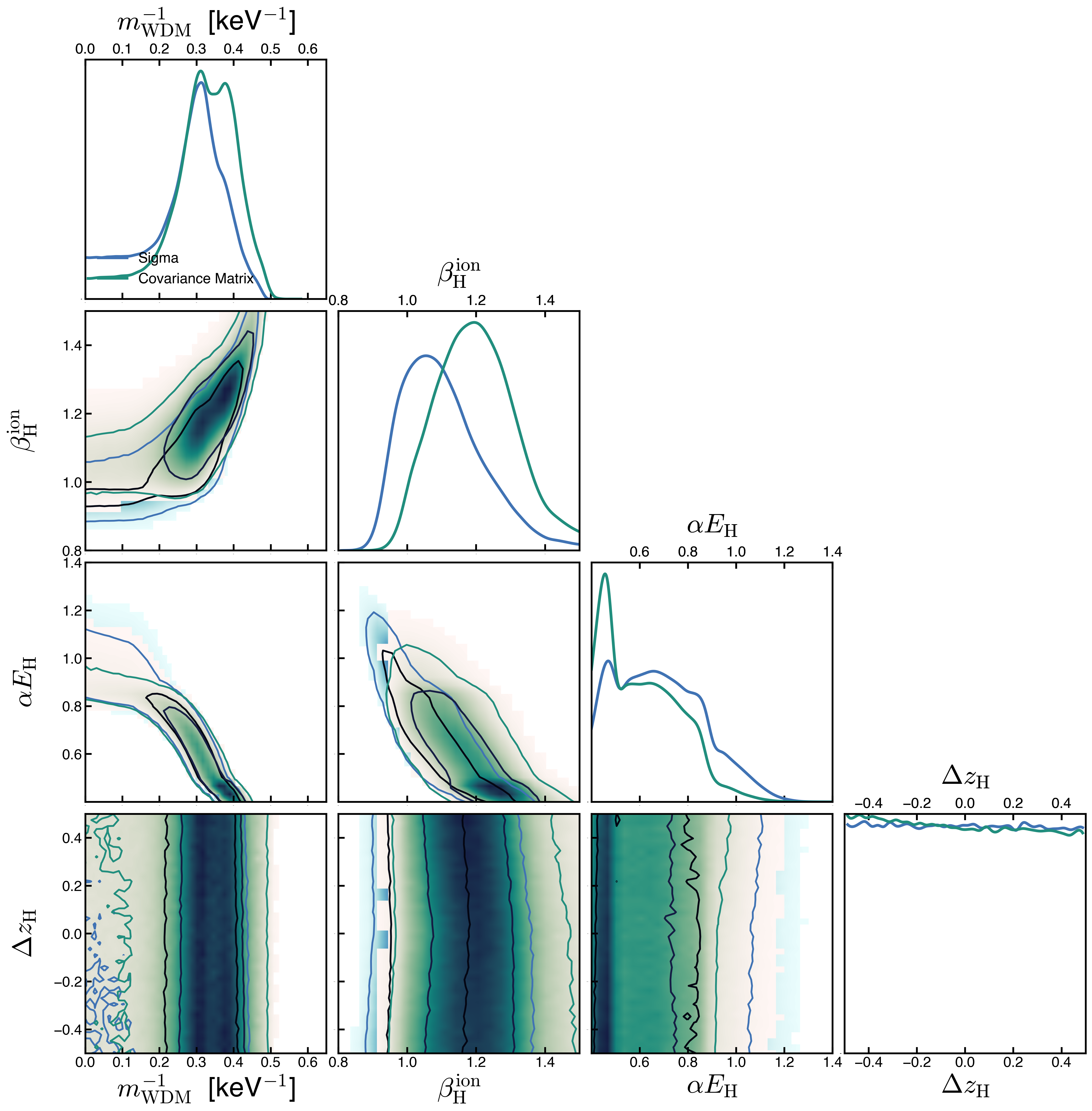
Fit only to \(z=5.0\)
Covariance from the simulations
Now I measure the effect of using the covariance matrix from the models which I rescale to have the same \(sigma\) as the data by applying the equation:
\[C_{i j}= C_{i j}^{s i m} \frac{ \sqrt{C_{i i}^{\text {data }} C_{j j}^{\text {data }}} }{\sqrt{C_{i i}^{s i m} C_{j j}^{s i m}}}\]I chose the 16 closest models from which I measure the rescaled covariance matrix and I use that to do the MCMC fit.
The parameters for the chosen models are the combinations of the following:
\(m_{\mathrm{WDM}}\): [ 3.0, 5.0 ] keV
\(\beta_{\mathrm{H}}^{\mathrm{ion}}\): [ 1.0, 1.4 ]
\(\alpha E_{\mathrm{H}}\): [ 0.5, 0.9 ]
\(\Delta z_{\mathrm{H}}\): [-0.5, 0.5]
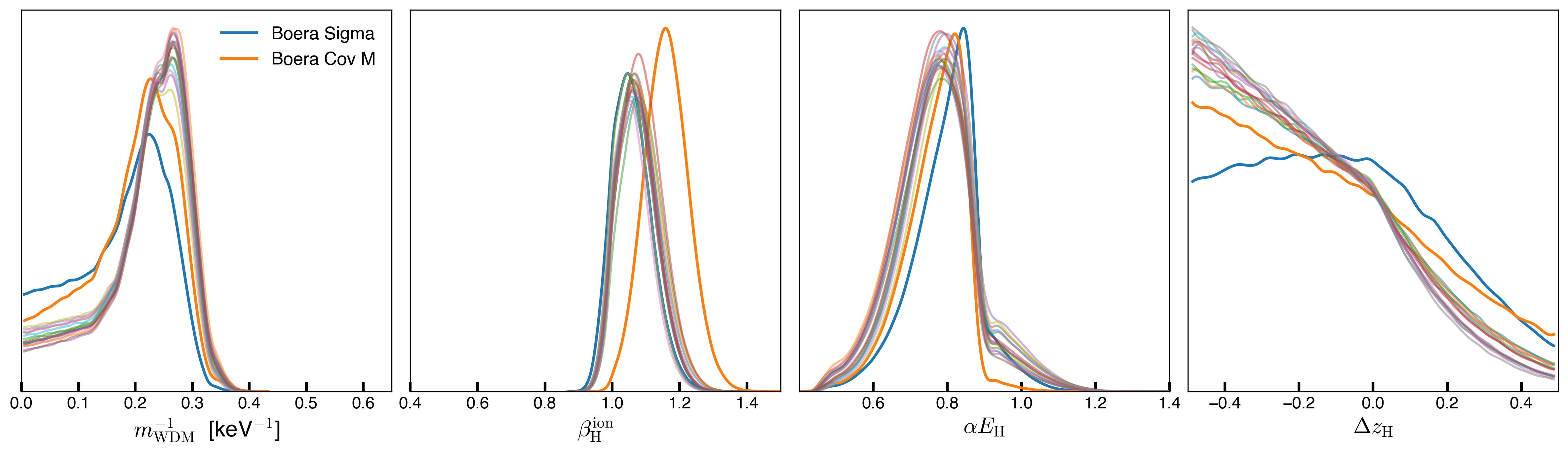
The marginalized distributions for the fits from the 16 covariance matrices is shown below:
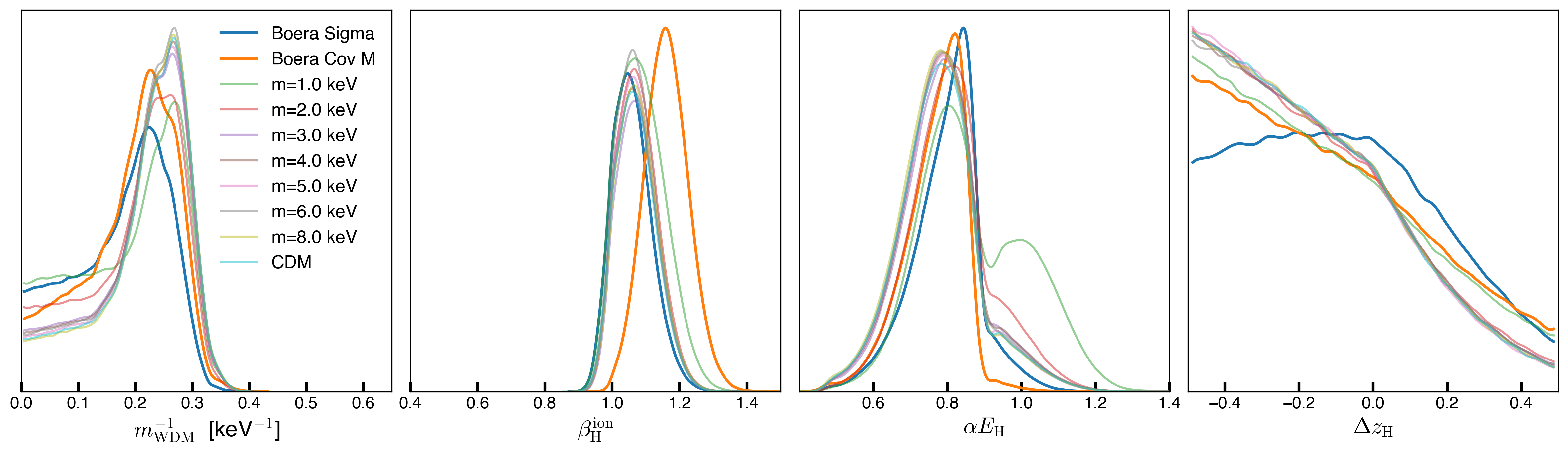
Now I fix the UVB parameters to those closest to the best-fit and use the covariance matrix obtained from the different different \(m_\mathrm{WDM}\) simulations.
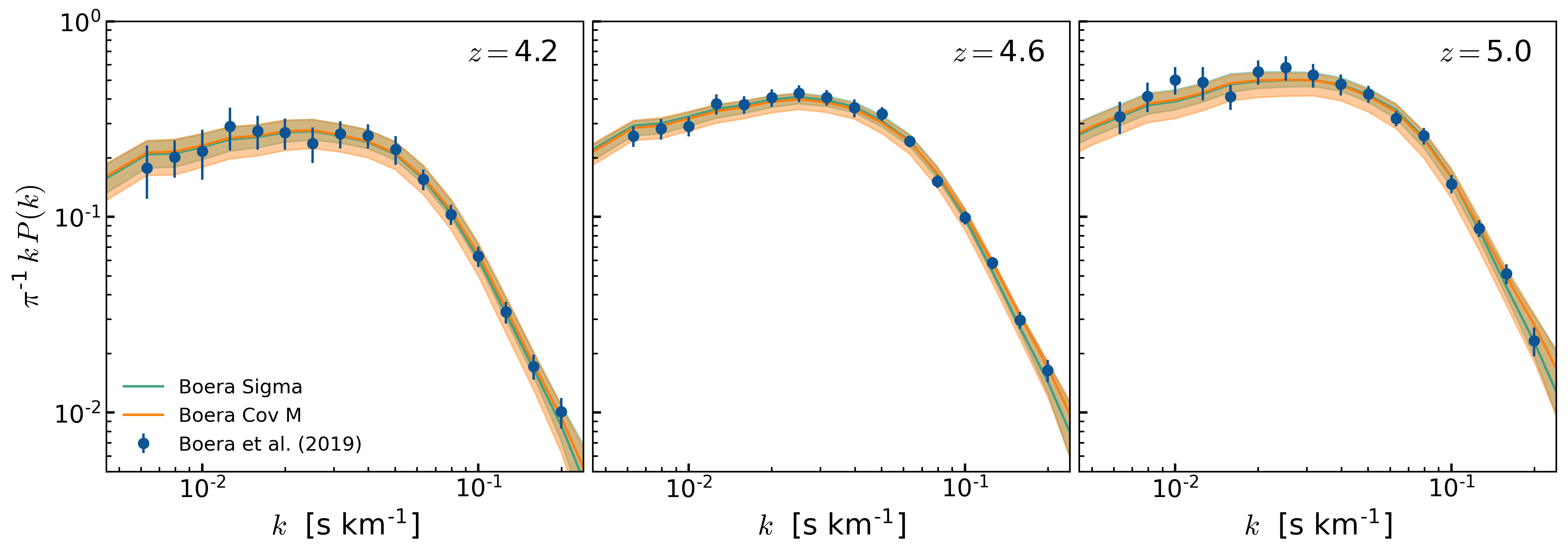
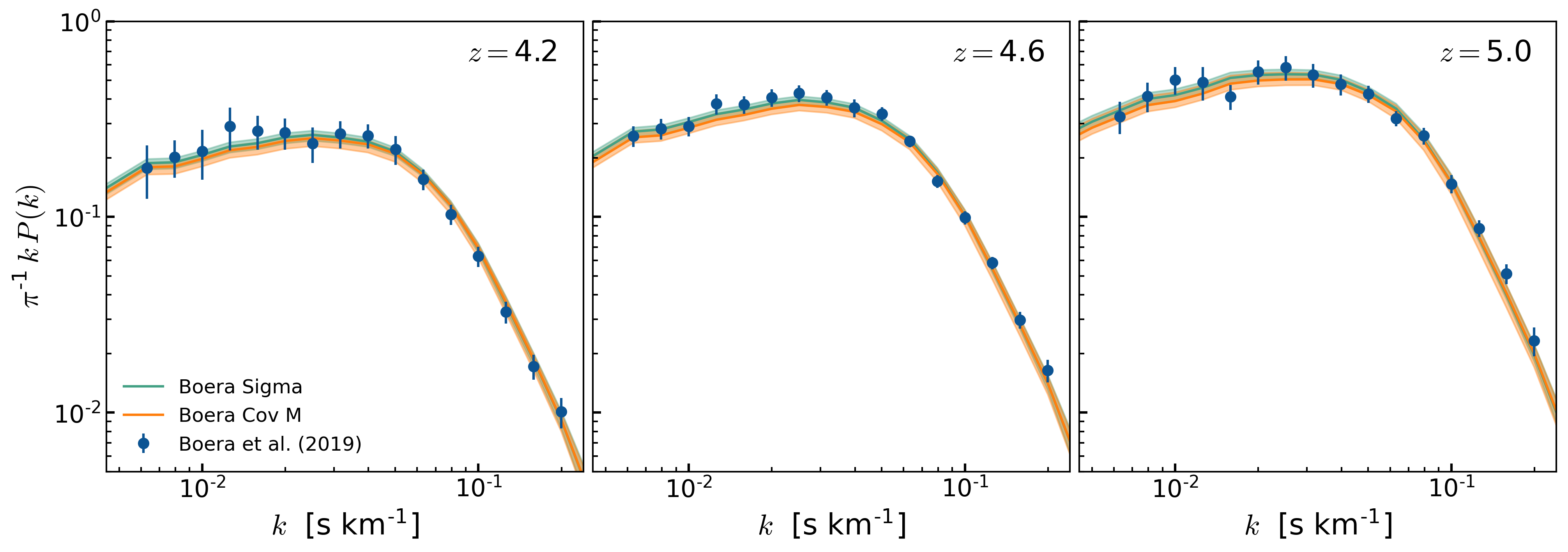
Marginalized Power Spectrum
Now I show the marginalized Power Spectrum from fitting the three redshifts simultaneously using the Covariance Matrix from Boera el al. and also just using \(\sigma\).
Now the same but fitting each redshift independently.