Cholla Chemistry solver compared to Grackle Revised

After rewriting the solver to closely follow the methodology from Grackle the results are very good.

Single zone test

First I compare a “single zone” test where the simulation is a small box with uniform density, zero velocities and uniform temperature. I compare the same simulation but in one case I use Grackle for the Chemistry/Cooling and for the other case I use the solver that I have implemented into Cholla.

The evolution of the temperature and the abundances of the chemical species are shown below:

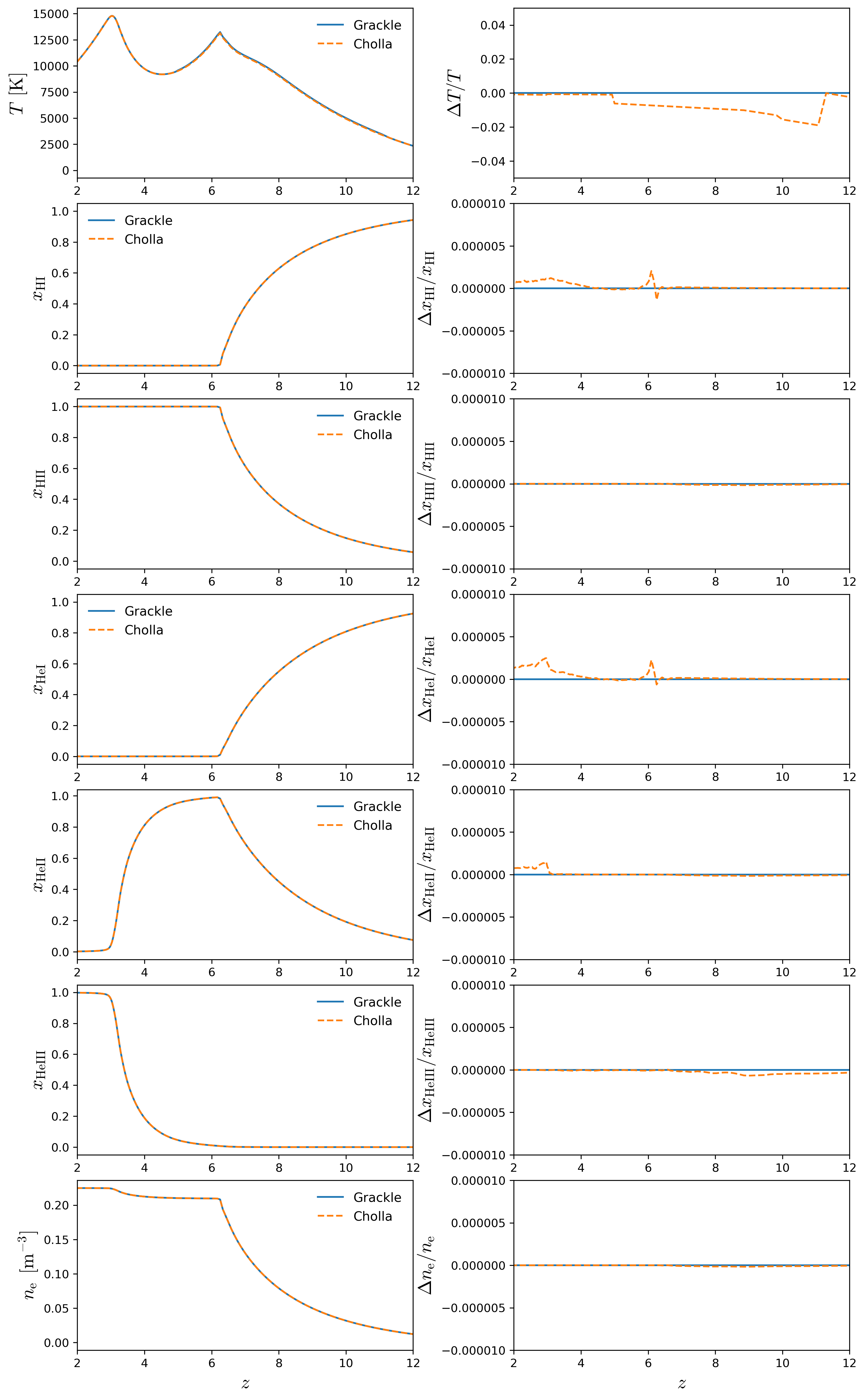
There are some small differences around 2% in the temperature. The ionization states of H and He seem extremely close showing differences smaller than 0.0001% !!!

Density-Temperature distribution

Now I run a full cosmological simulation ( $L=50 h^{-1} \mathrm{Mpc}$, $N=256^3$ ). Below I compare the evolution of the density temperature distribution

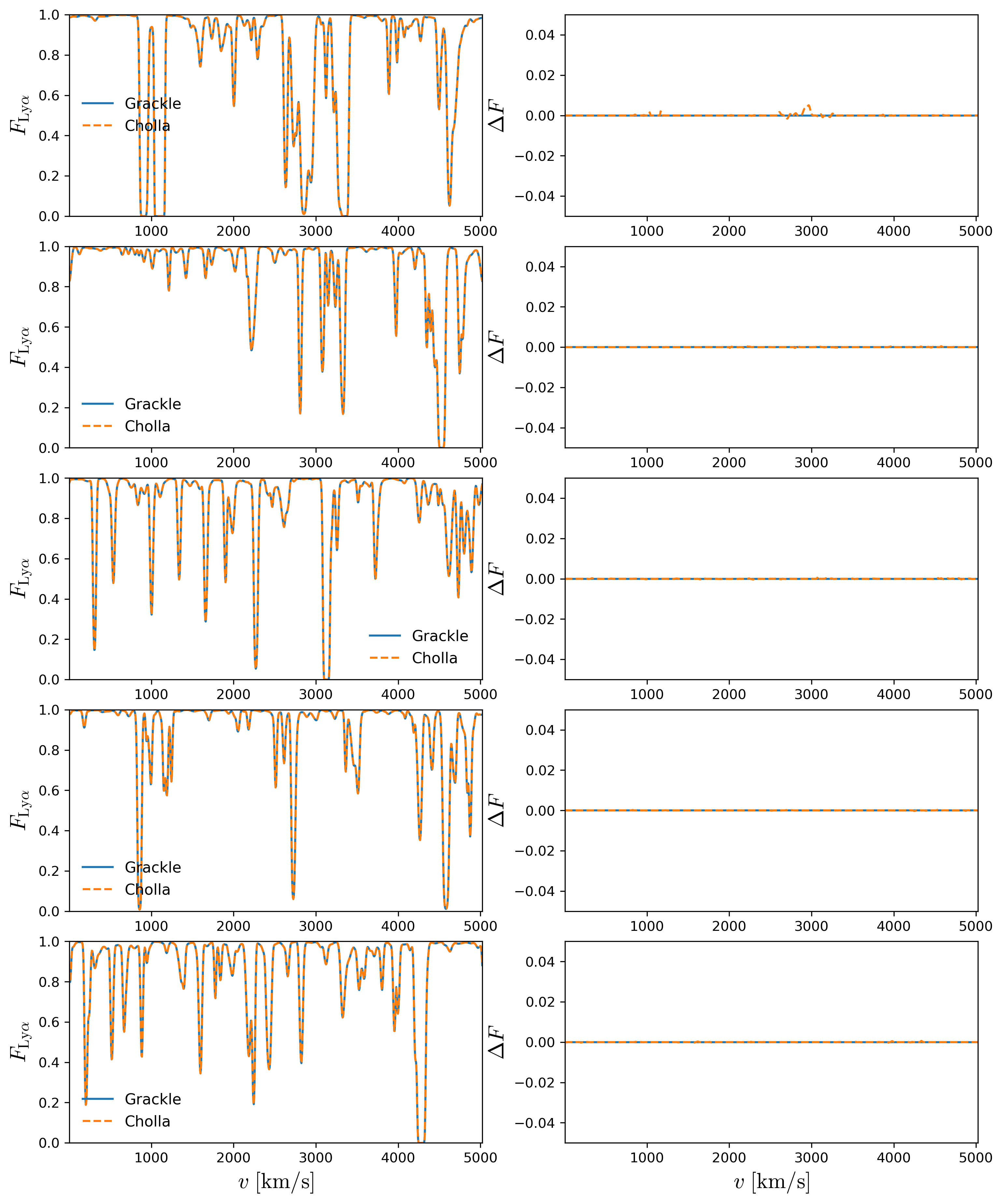
Lya Transmitted Flux along skewers

From a higher resolution simulation ( $L=50 h^{-1} \mathrm{Mpc}$, $N=1024^3$ ), I measure the Lya transmitted flux along some skewers crossing the box, the comparison for several redshift values is below

$z = 5.0$

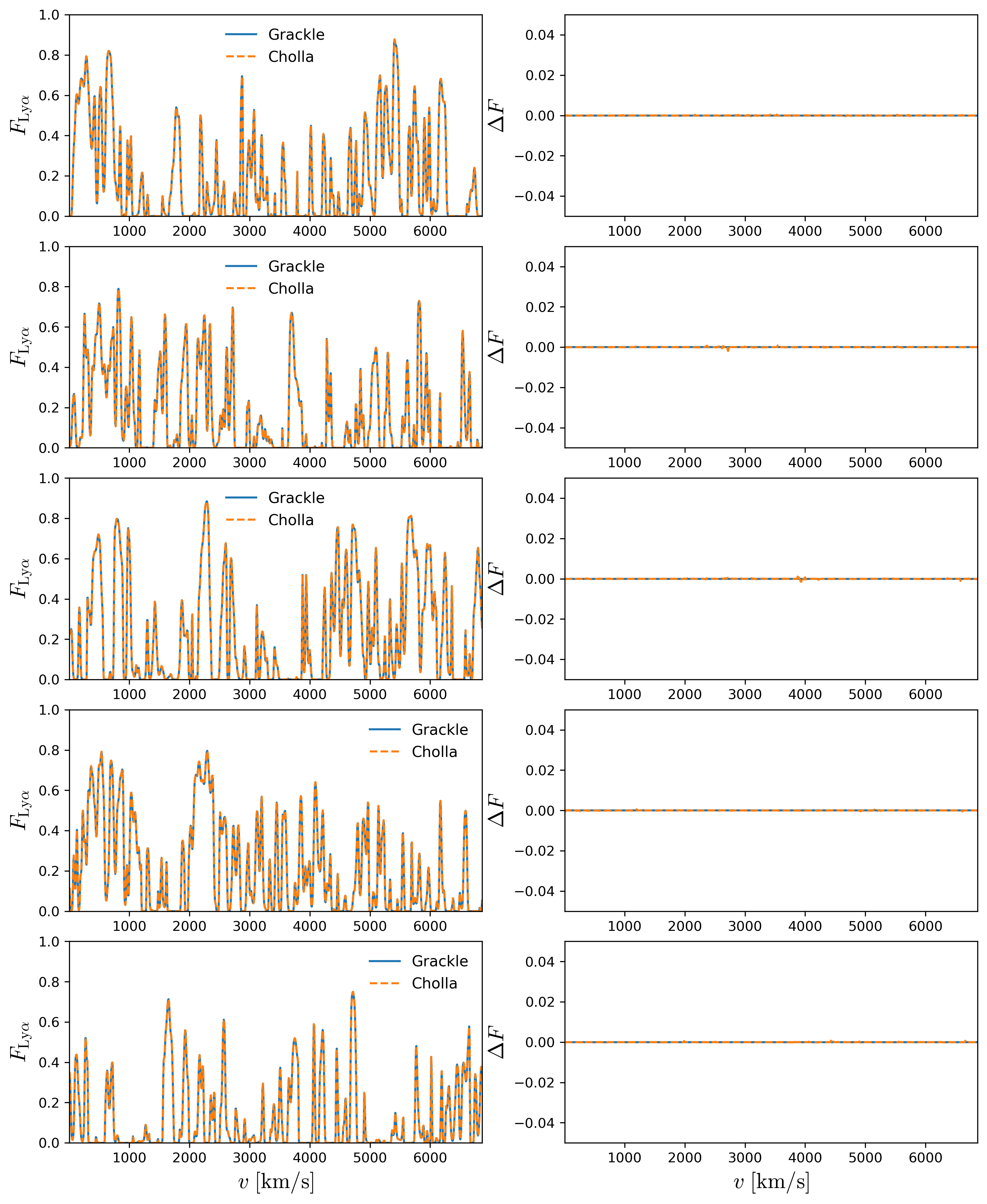
$z = 4.0$

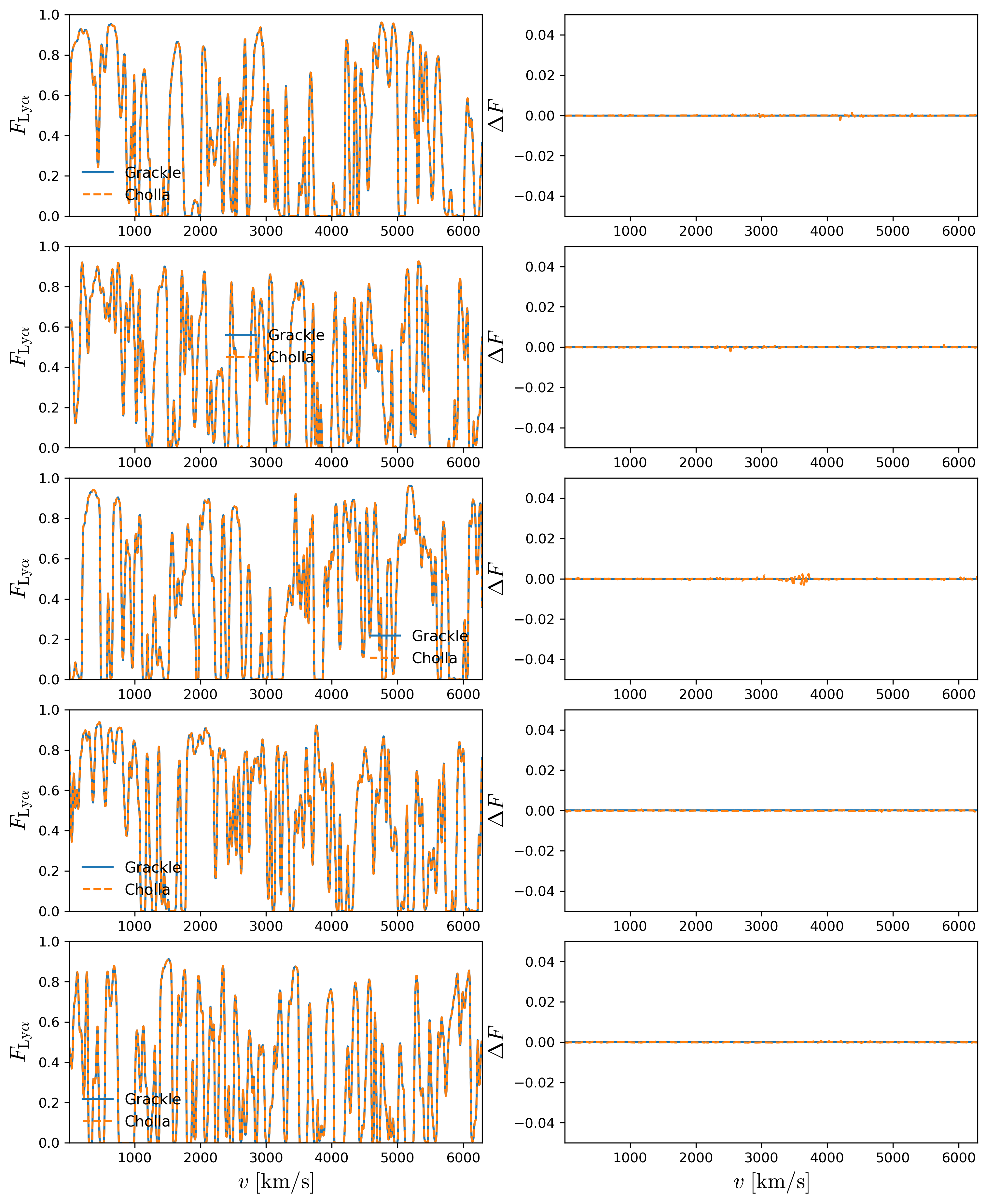
$z = 3.0$

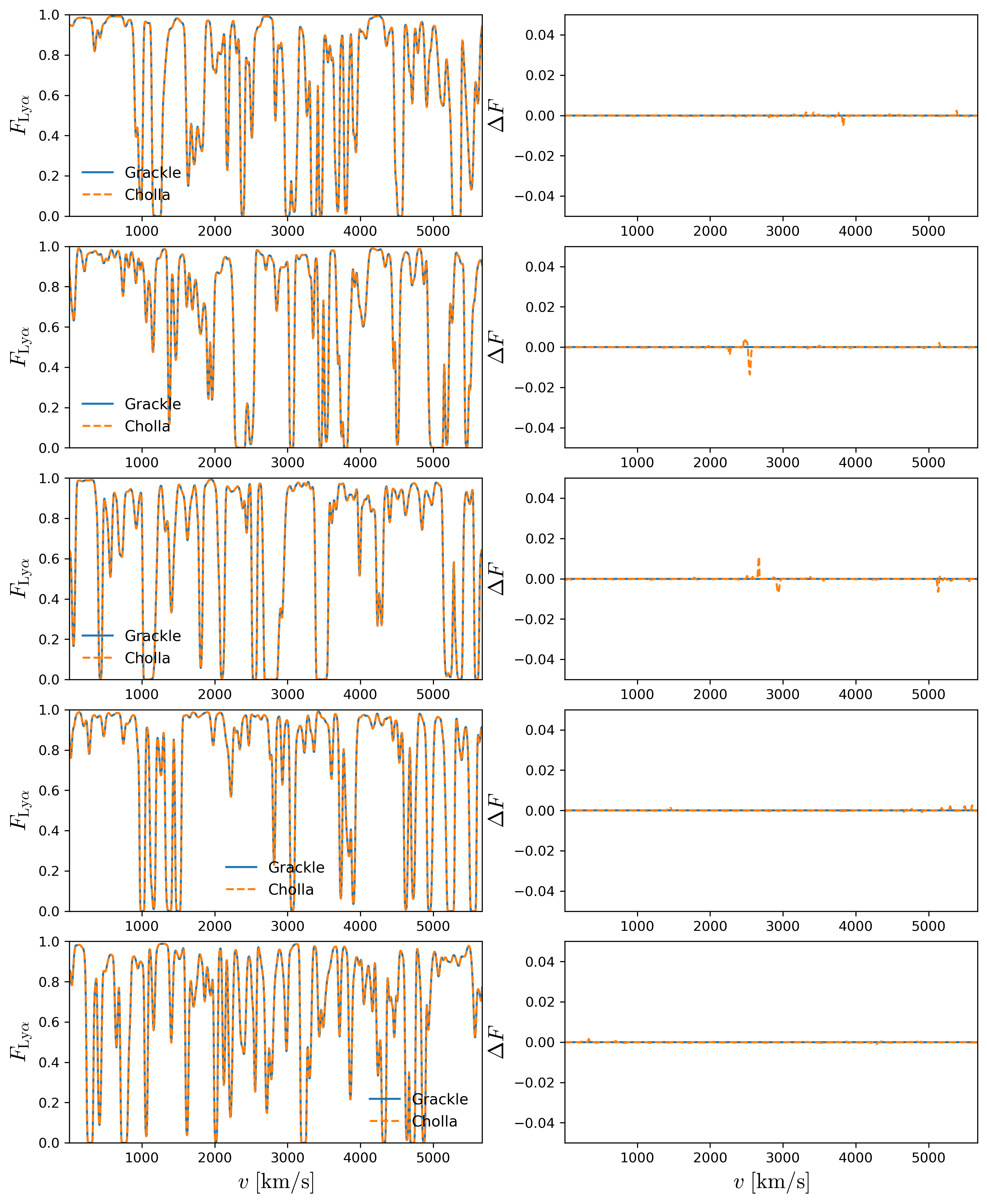
$z = 2.0$

Lya Flux Power Spectrum

From the ( $L=50 h^{-1} \mathrm{Mpc}$, $N=1024^3$ ) simulation, I measure the evolution of the Lya Flux Power Spectrum, the comparison is below:

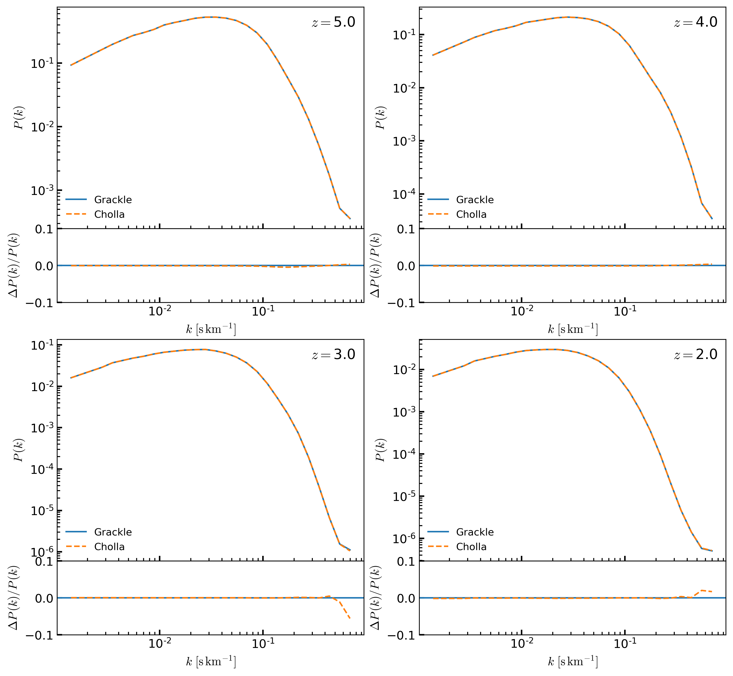
Only small differences on the highest $k$ bin.

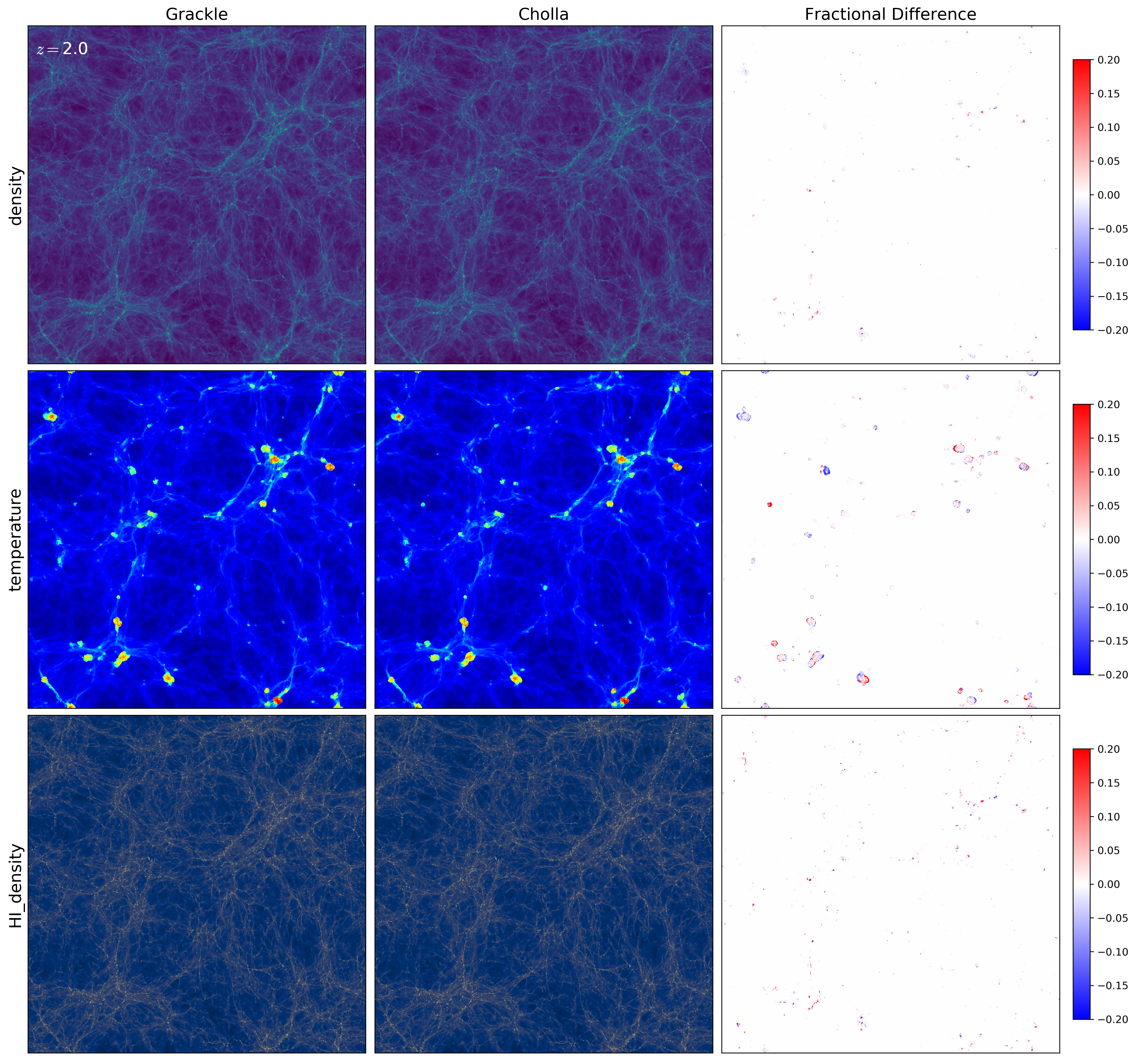
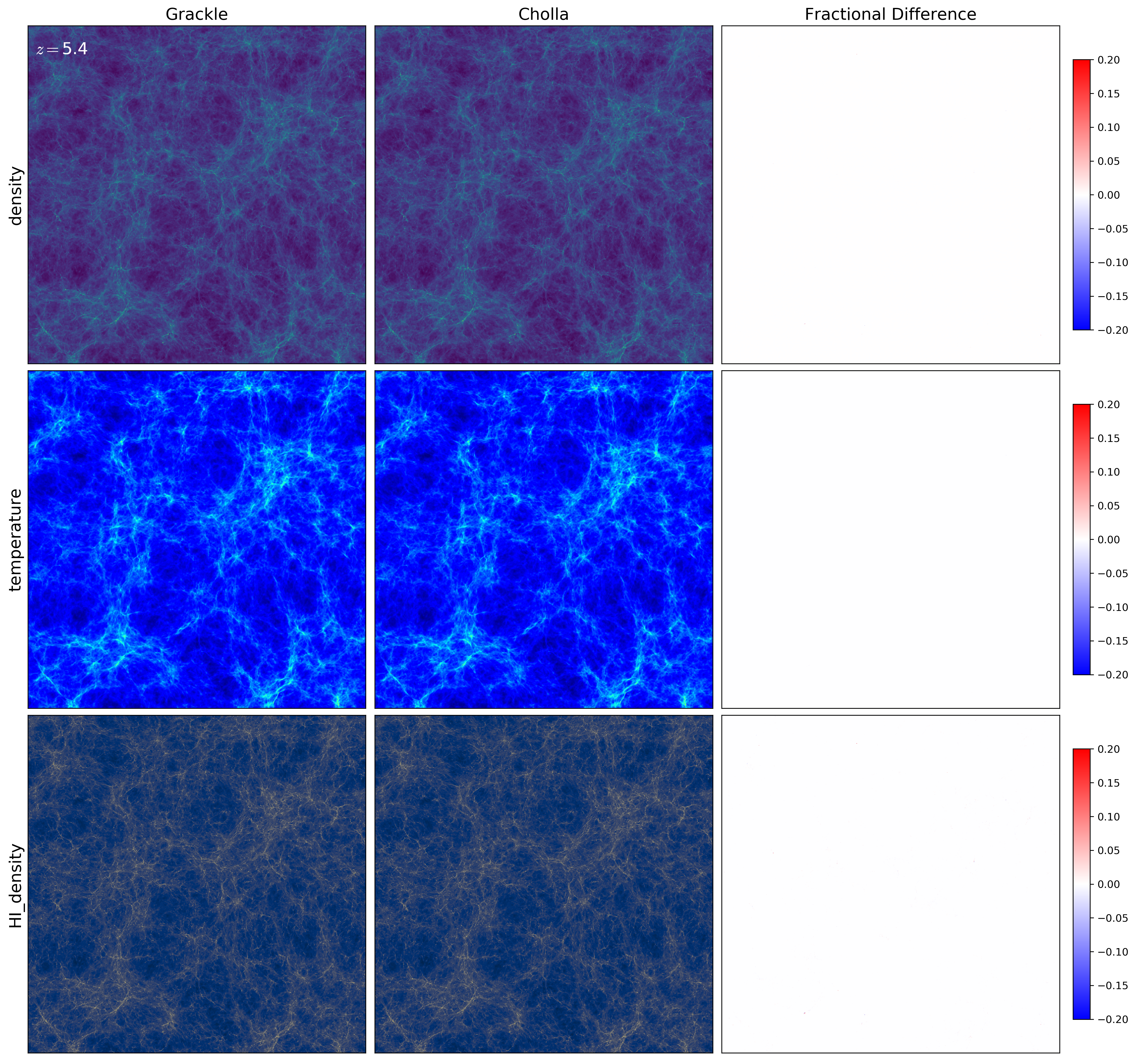
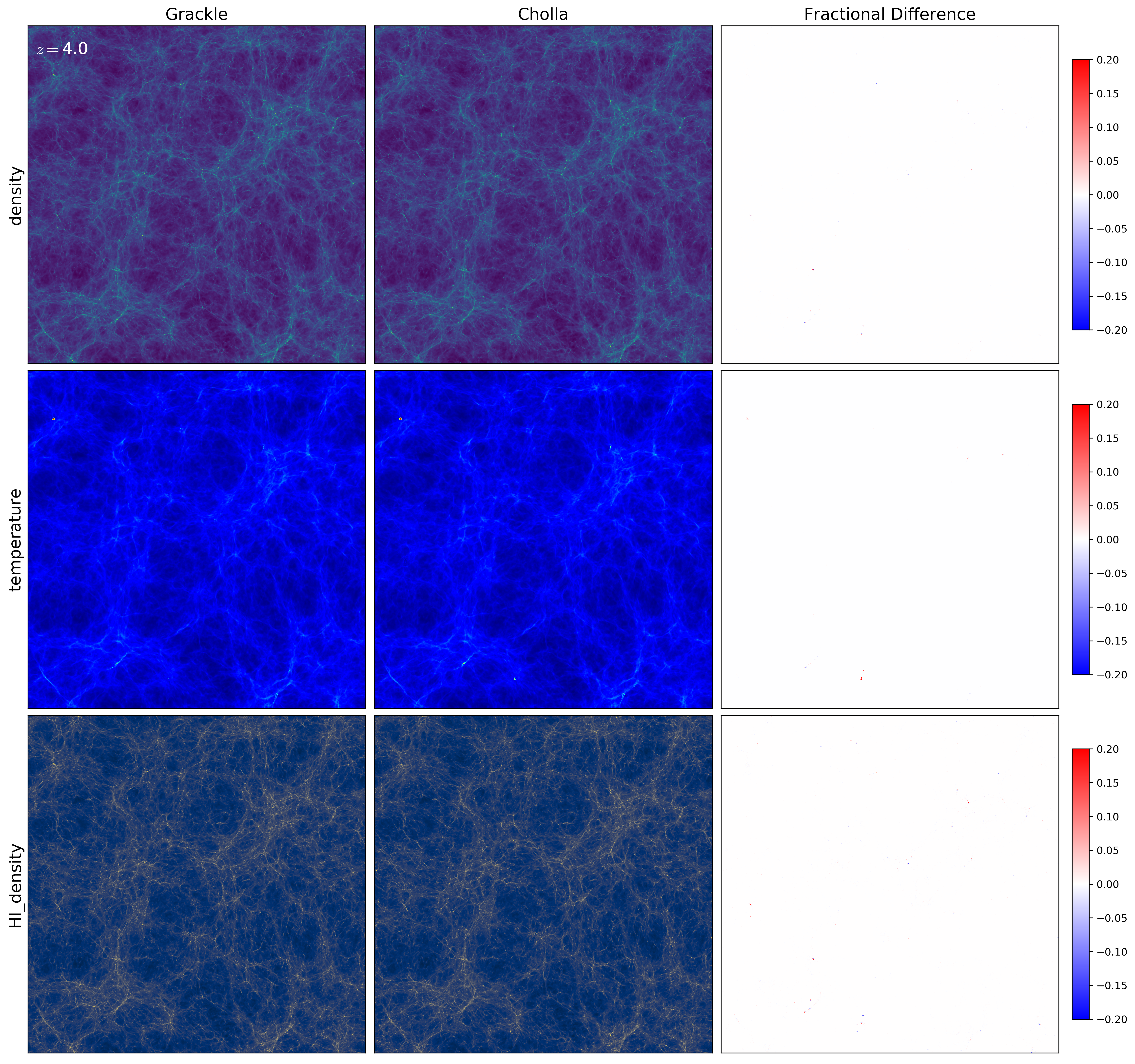
Slices from the Simulations

z=5.4

z=4.0

z=3.0

z=2.0