Cholla Chemistry solver compared to Grackle
Single zone test
First I compare a “single zone” test where the simulation is a small box with uniform density, zero velocities and uniform temperature. I compare the same simulation but in one case I use Grackle for the Chemistry/Cooling and for the other case I use the solver that I have implemented into Cholla.
The evolution of the temperature and the abundances of the chemical species are shown below:
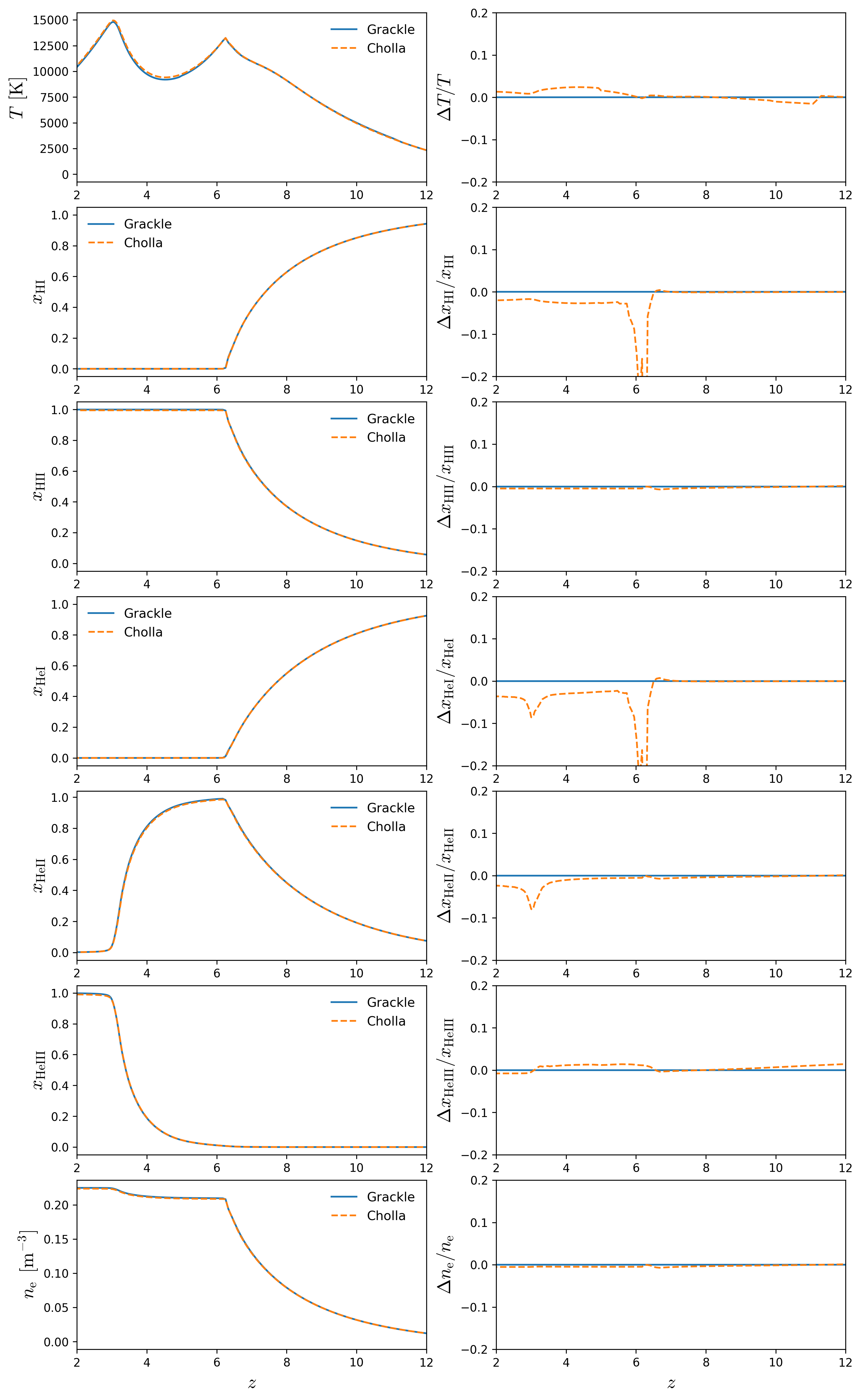
There are small differences in the temperature, this might be because the some differences in the Cooling rates used. Also some differences in the HI and HeI fractions are shown at \(z \sim 6\) these differences are at the end of Hydrogen reionization, and the reason could be that Grackle uses some special trick to handle the transition to photoionization equilibrium.
Density-Temperature distribution
Now I run a full cosmological simulation ( \(L=50 h^{-1} \mathrm{Mpc}\), \(N=256^3\) ). Below I compare the evolution of the density temperature distribution
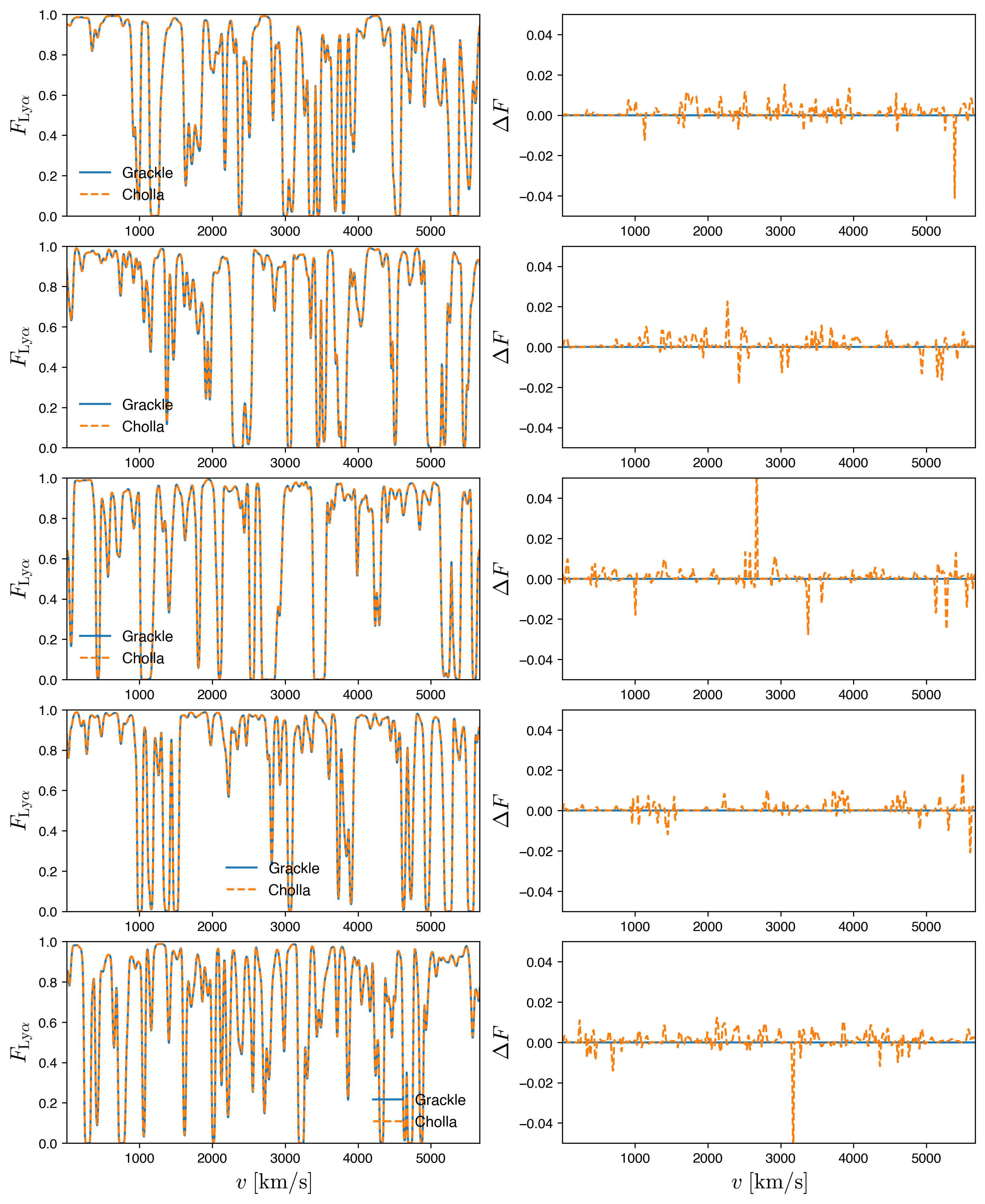
Lya Transmitted Flux along skewers
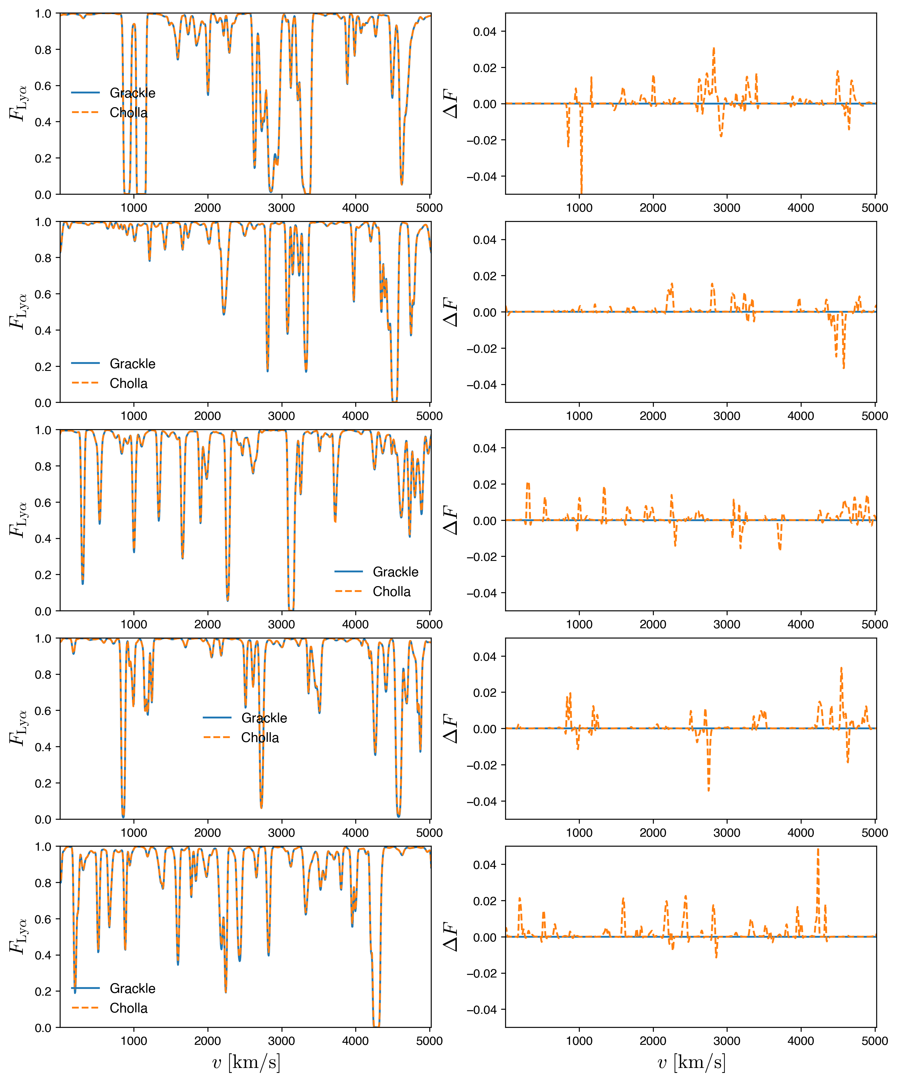
From a higher resolution simulation ( \(L=50 h^{-1} \mathrm{Mpc}\), \(N=1024^3\) ), I measure the Lya transmitted flux along some skewers crossing the box, the comparison for several redshift values is below
\(z = 5.0\)
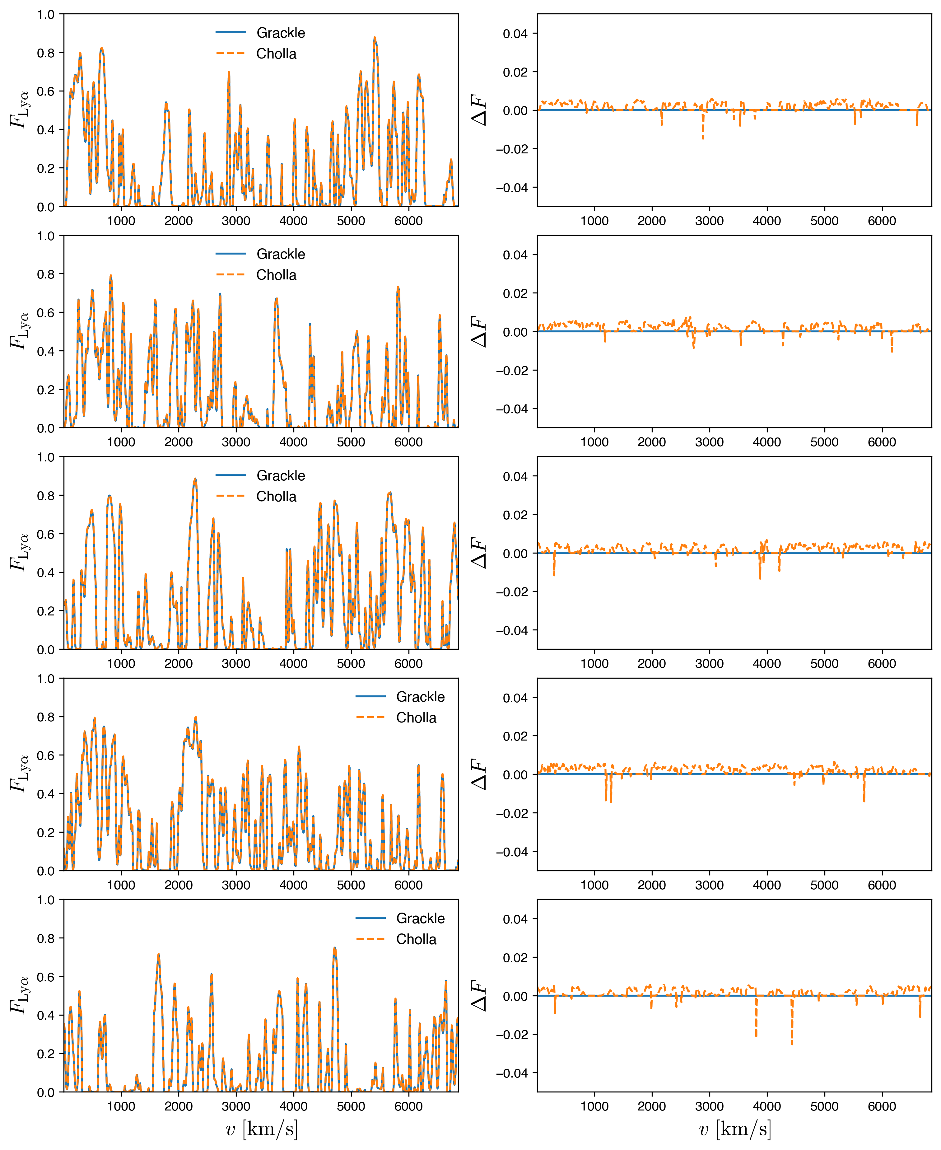
\(z = 4.0\)
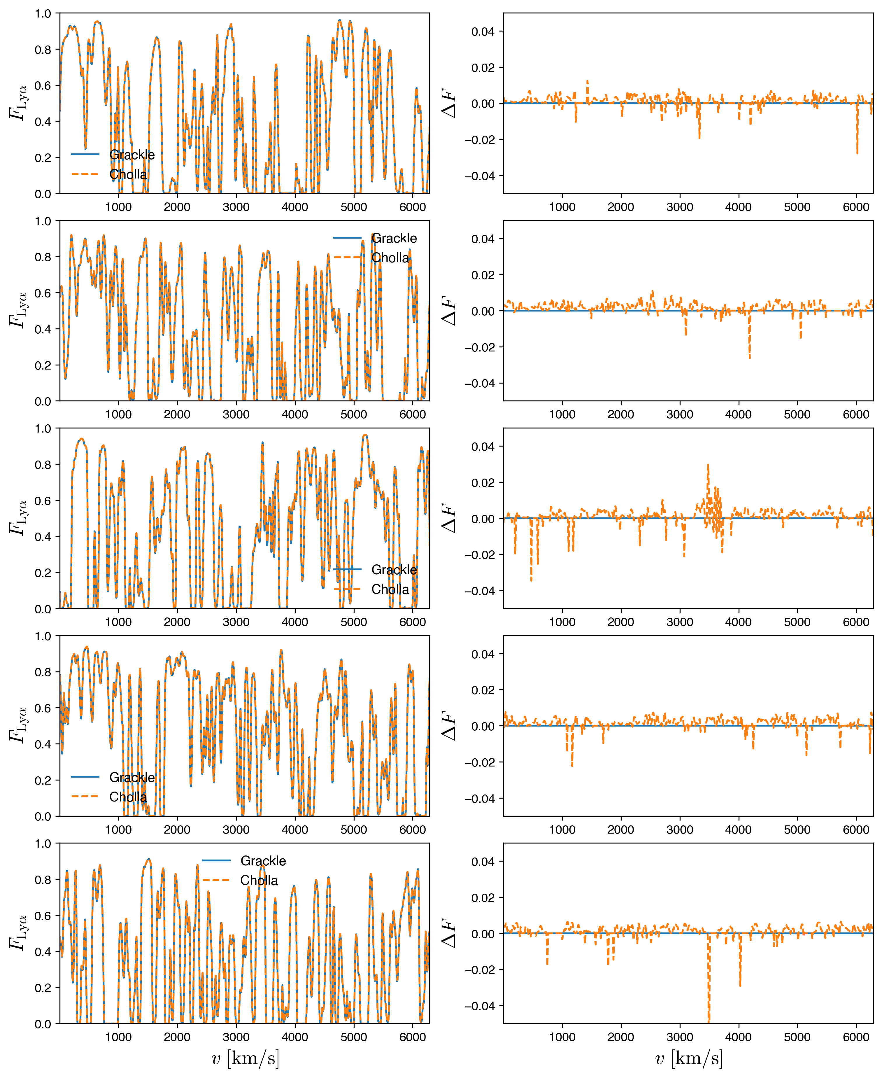
\(z = 3.0\)
\(z = 2.0\)
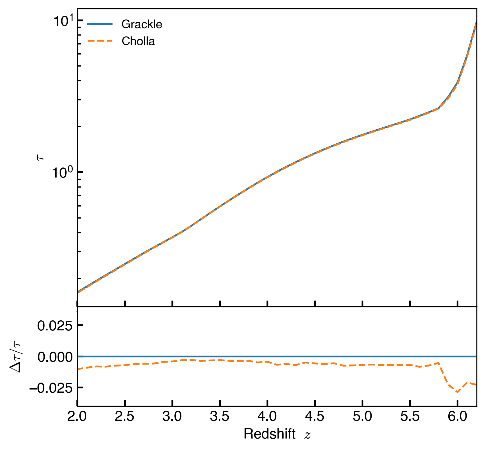
Lya Effective Optical Depth
From the ( \(L=50 h^{-1} \mathrm{Mpc}\), \(N=1024^3\) ) simulation, I measure the evolution of the Lya Effective Optical Depth, the comparison is below:
Lya Flux Power Spectrum
From the ( \(L=50 h^{-1} \mathrm{Mpc}\), \(N=1024^3\) ) simulation, I measure the evolution of the Lya Flux Power Spectrum, the comparison is below:
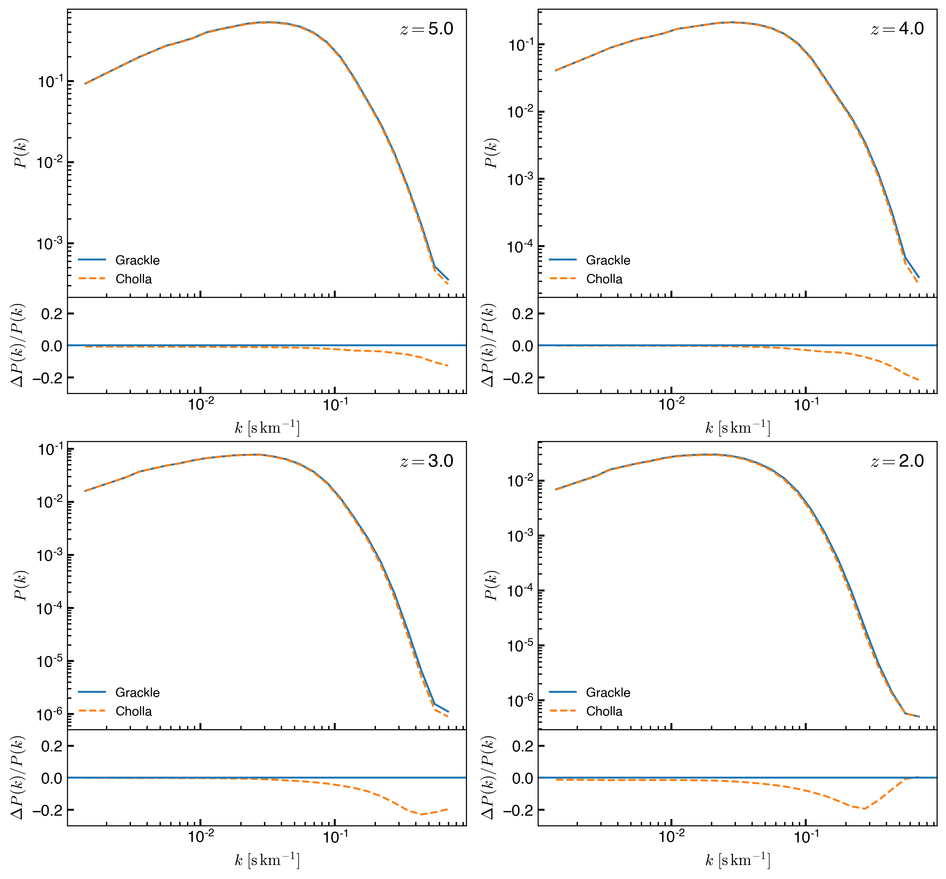
There are some differences as large as \(\sim 25\%\) on small scales.
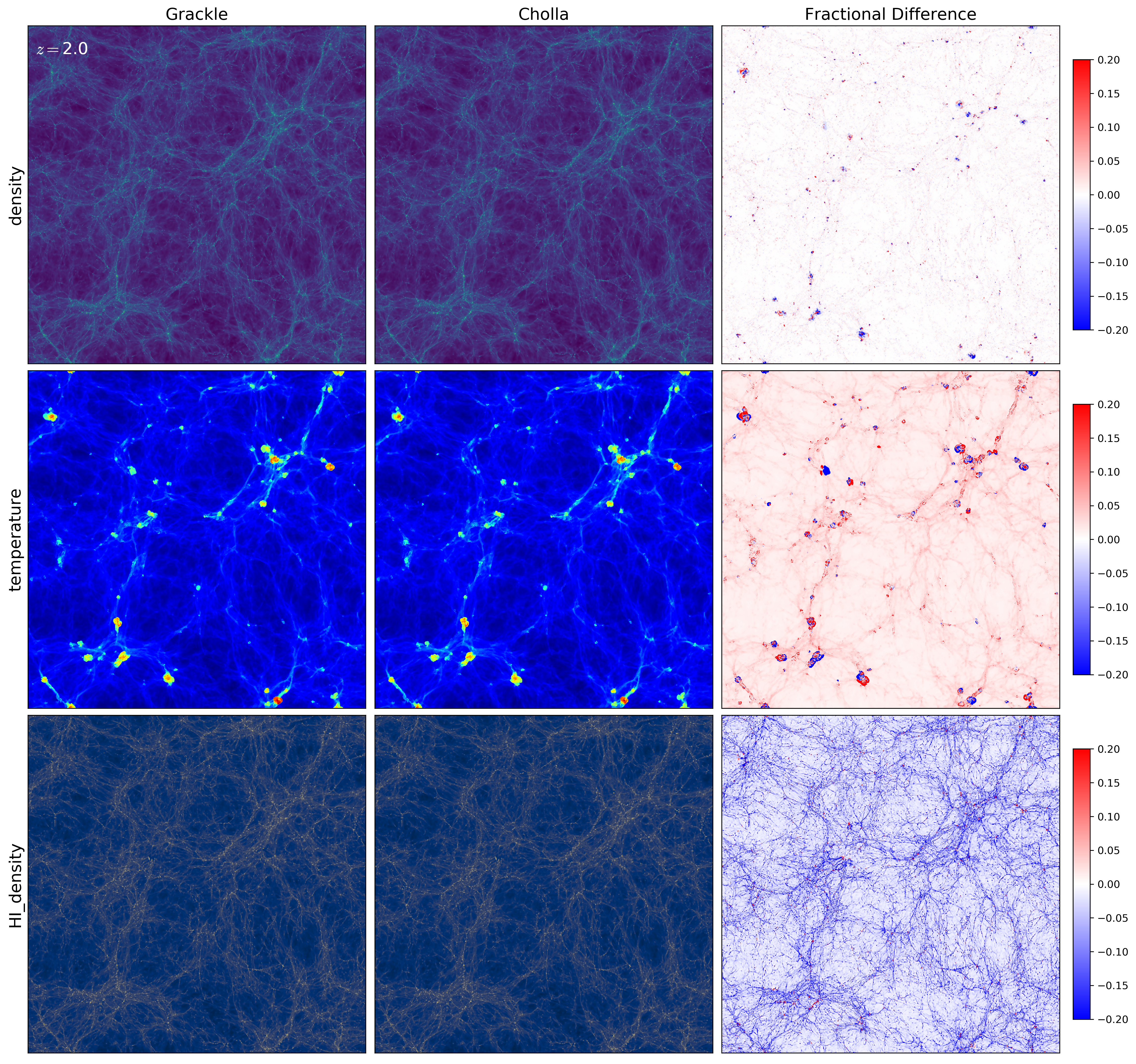
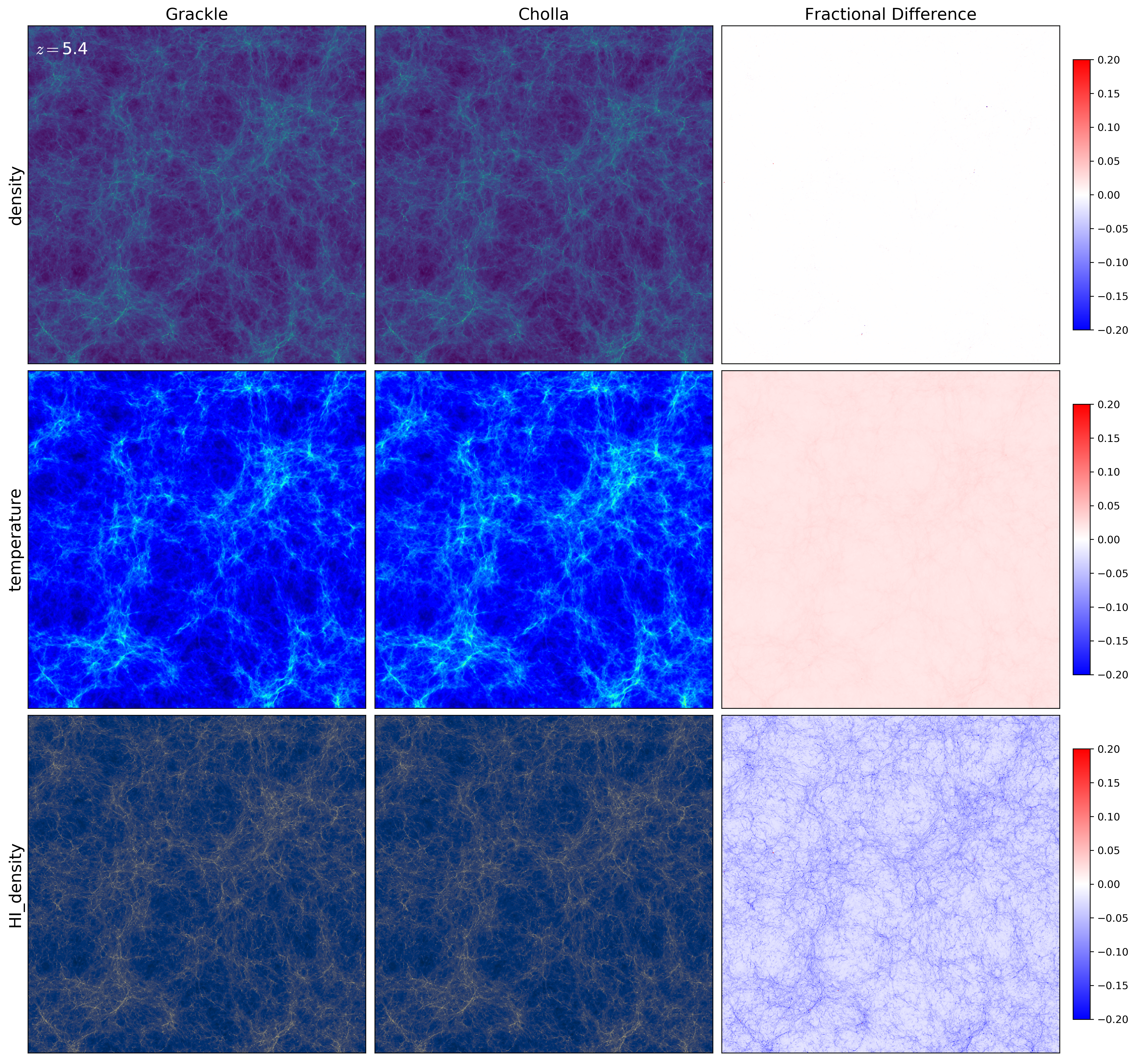
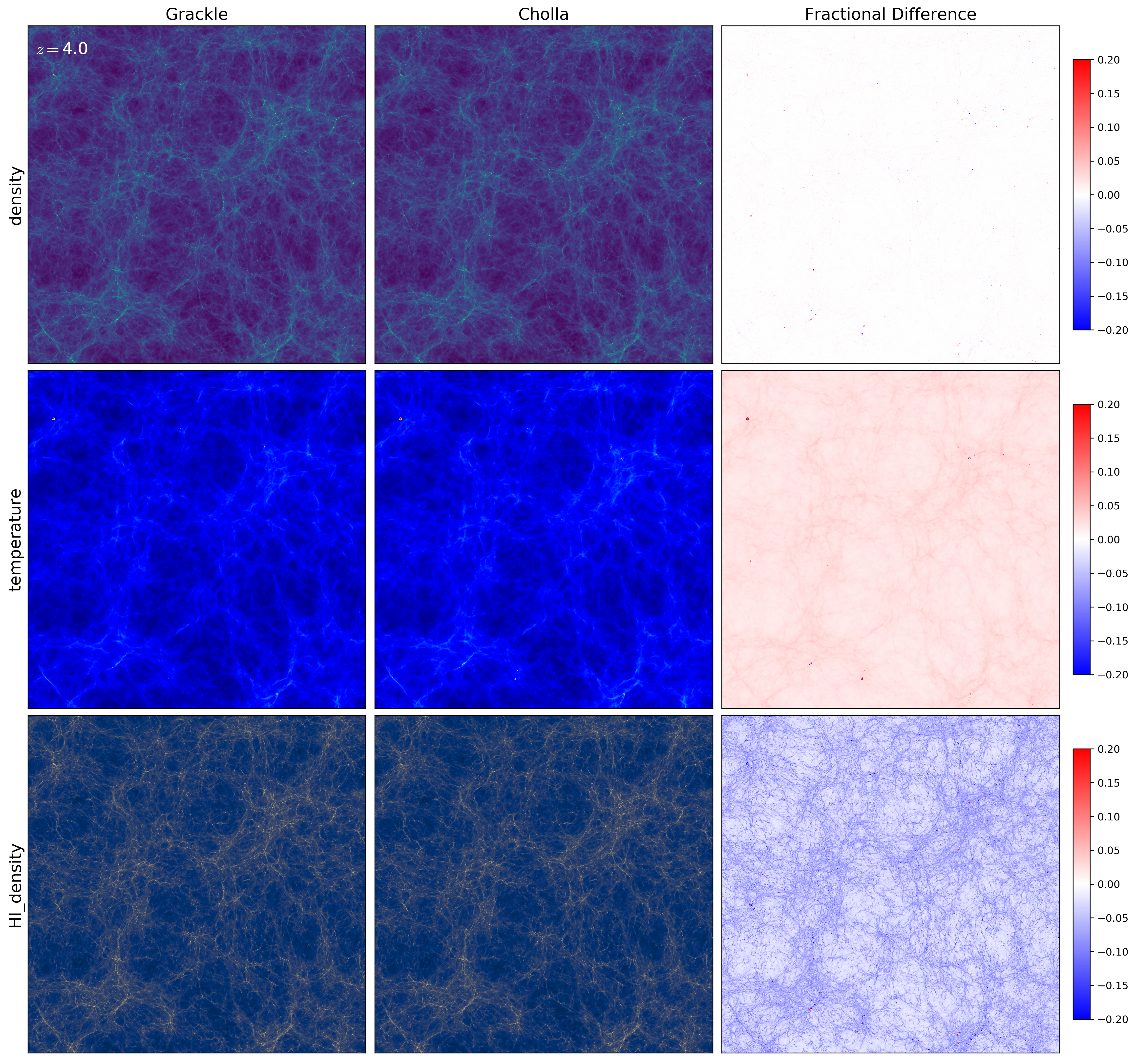
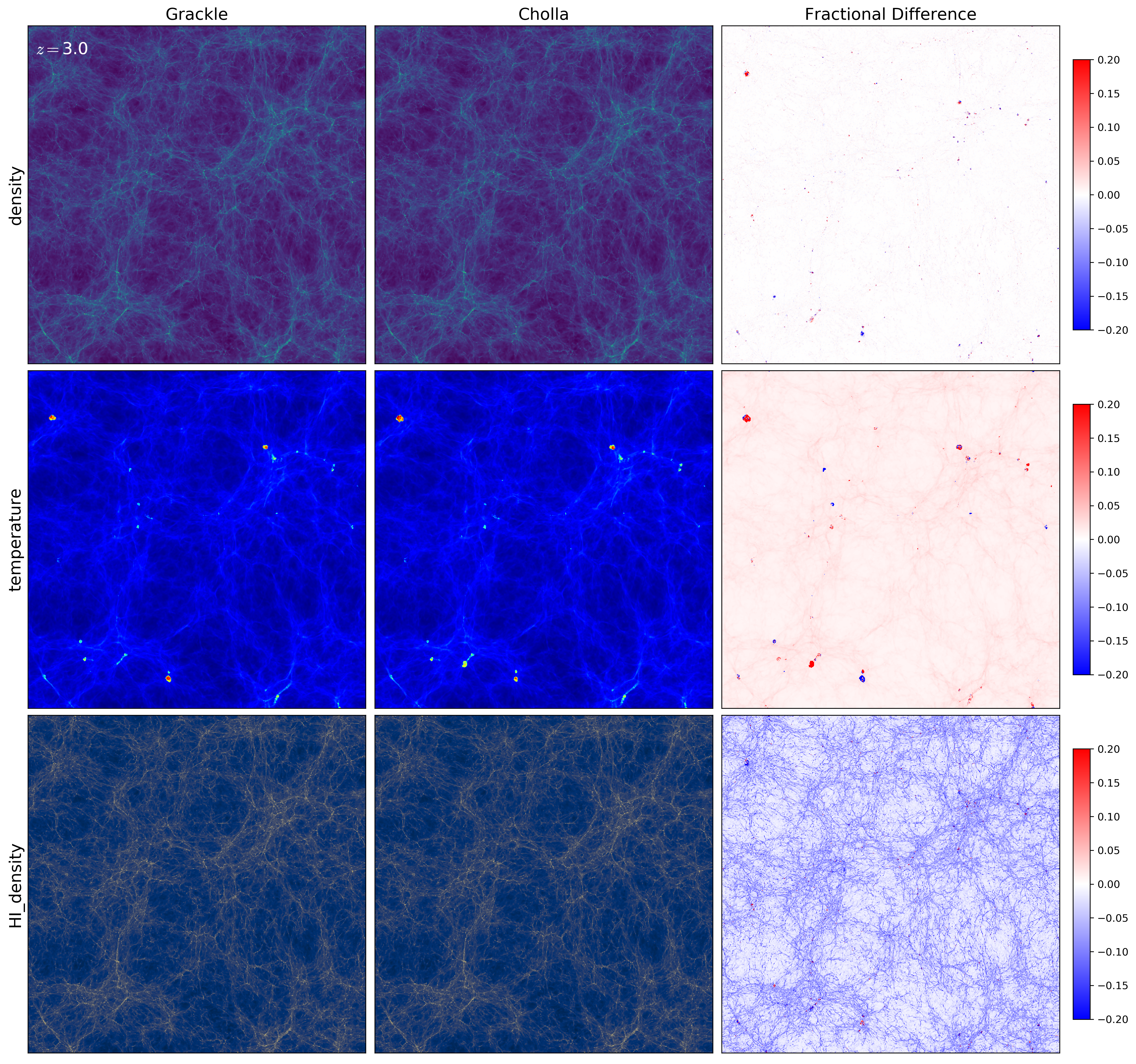
Slices from the Simulations
z=5.4
z=4.0
z=3.0
z=2.0