Modeling The Density-Temperature Distribution
Evolution of the density-temperature distribution from the 100 Mpc/h \(2048^3\) box using our new Rescaled P19 model:
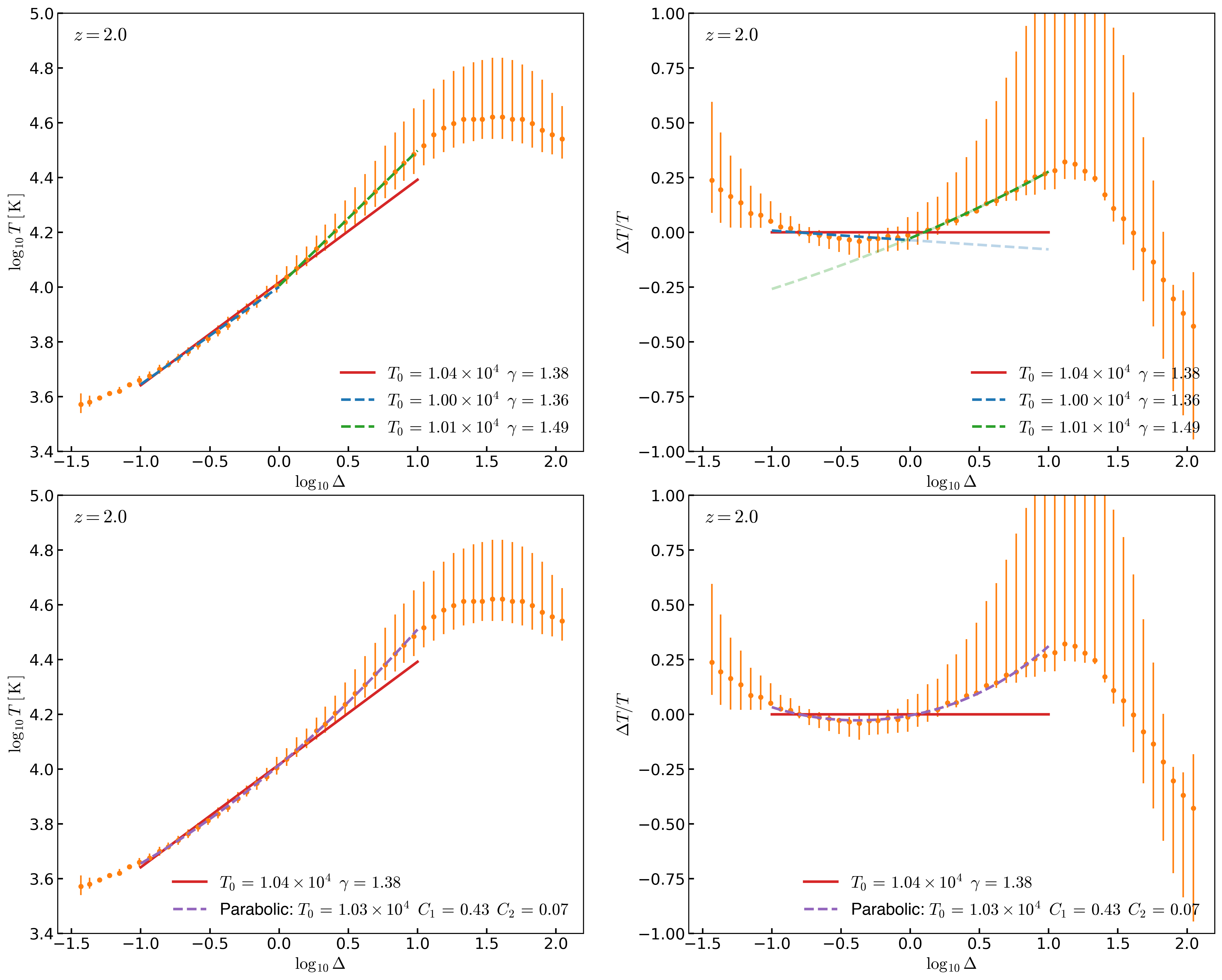
\[\beta_{\mathrm{He}} = 0.44\] \[\beta_{\mathrm{H}} = 0.78\] \[\Delta z_{\mathrm{He}} = 0.27\] \[\Delta z_{\mathrm{H}} = 0.05\]From the Density-Temperature distribution I measure the 65% Highest Probability Interval for the temperature at constant overdensity, from those I get the temperature values as a function of overdensity wich I use to fit different models:
Top Panels:
-
Red Line: This is the original fitting method. Fit a lineal model in log-log space from in the interval \(\Delta = [-1, 1]\)
-
Blue Dashed Line: Fit a lineal model in log-log space from in the interval \(\Delta = [-1, 0]\)
-
Green Dashed Line: Fit a lineal model in log-log space from in the interval \(\Delta = [0, 1]\)
Left Panel: Shows the fractional difference with respect to the original fit ( red line )
Bottom Panels:
-
Red Line: This is the original fitting method. Fit a lineal model in log-log space from in the interval \(\Delta = [-1, 1]\)
-
Pourple Dashed Line: Fit a quadratic model in log-log space from in the interval \(\Delta = [-1, 1]\)
Now I show the same fits for different redshifts
Clearly a single liner model doesn’t fit the two intervals \(\Delta = [-1, 0]\) and \(\Delta = [0, 1]\) simultaneously, a broken power law is a better fit and the quadratic fit also is a good fit.