Flux Power Spectrum Comparison to Data Quantified

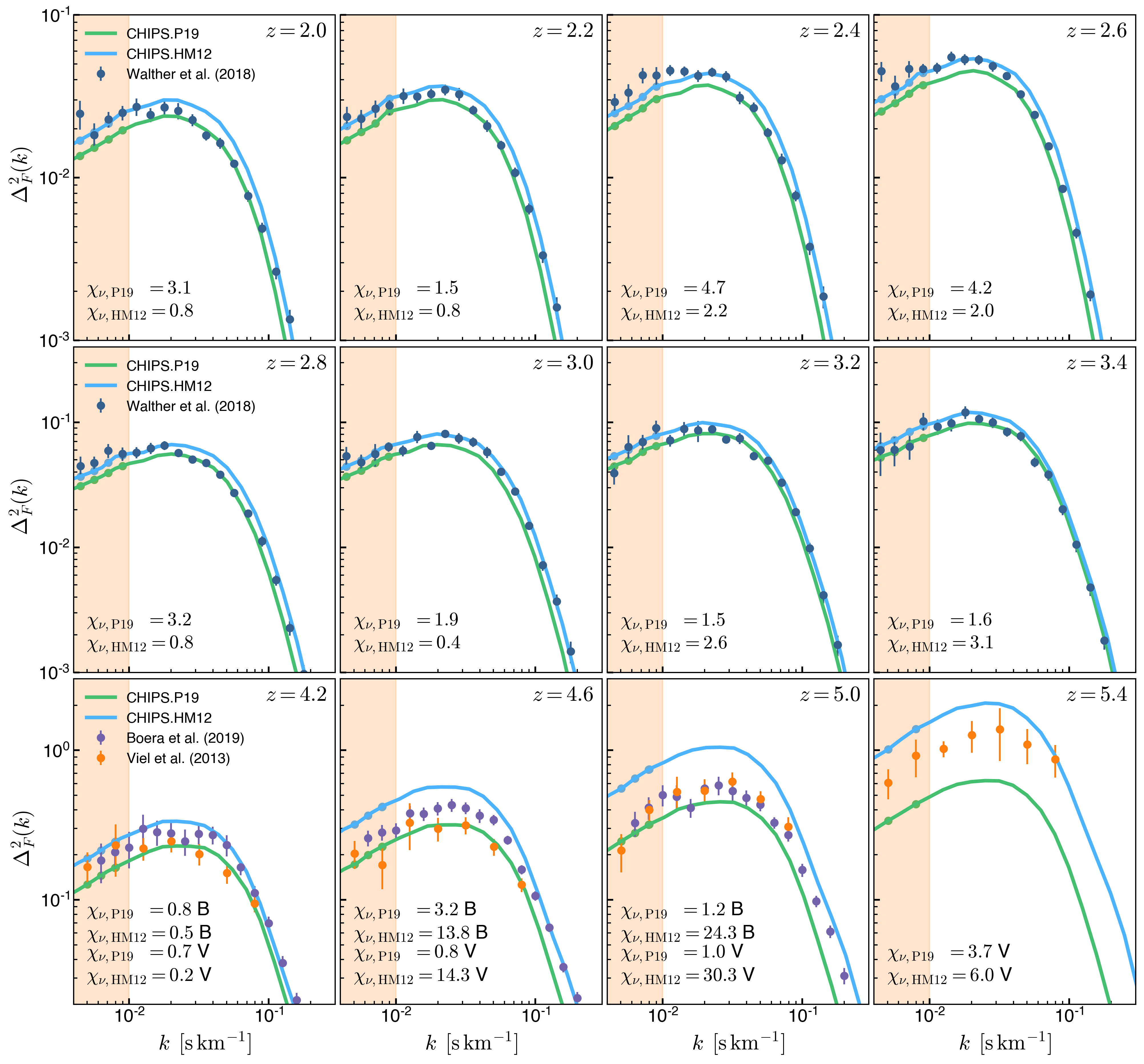
Figures below show the differences in the Flux Power Spectrum measured in our simulations compared to the observational data. The differences are quantified by $\chi^2$ defined as:

$$\chi^{2} = \sum_{i}^N \left[ \frac{ P(k_i)^{\mathrm{observ}} - P(k_i)^{\mathrm{model}} } { \sigma_i^{\mathrm{observ}} } \right]^{2}$$

The reduced error $\chi^2_{\nu, \mathrm{P19}}$ and $\chi^2_{\nu, \mathrm{HM12}}$ shown in the figures for each snapshot are computed as:

$$\chi^2_{\nu} = \frac{ \chi^2 }{ N } }$$

For the small scale comparison the scales selected are $0.01 \leq k \leq 0.1 \, \mathrm{s} \, \mathrm{km}^{-1}$ and the measurements of $\chi^2$ is computed separately for each of the observational data sets.

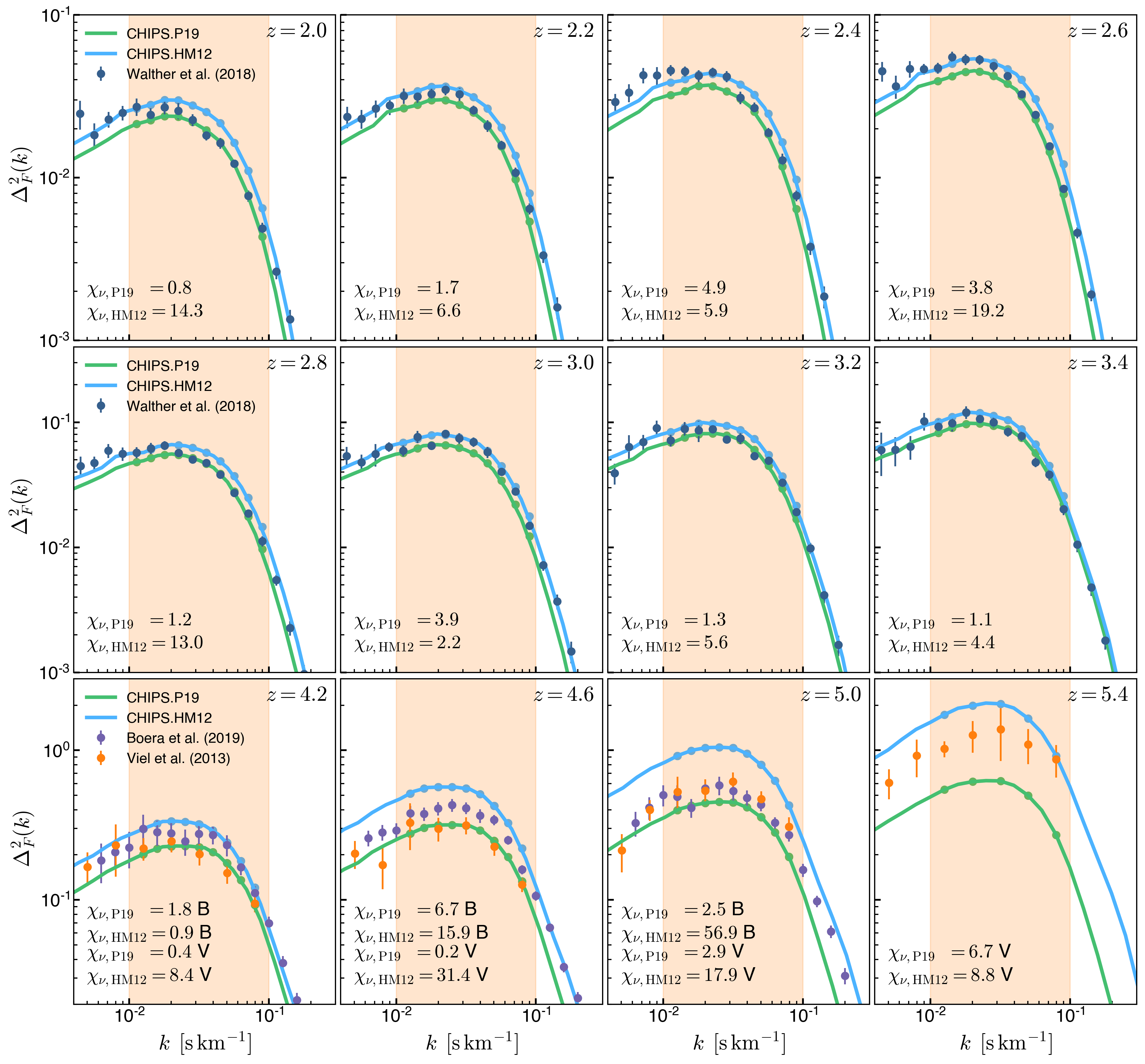
The distribution of $\chi^2_{\nu}$ for the two models is summarized in the following figure:

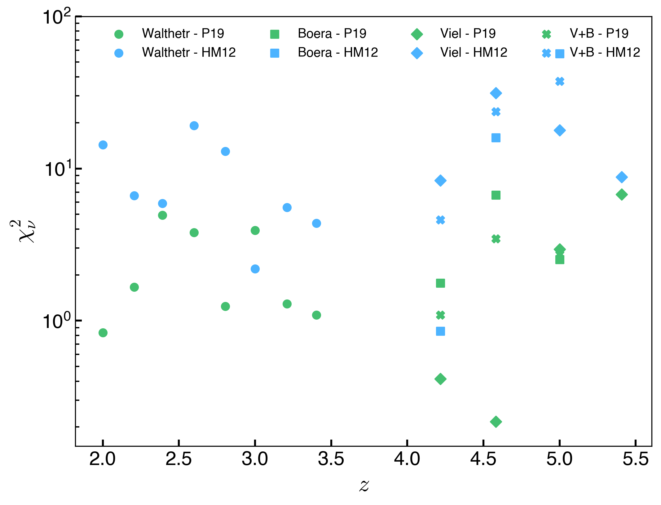
For $2\lesssim z \lesssim 4.5$, $\langle \chi^2_\nu \rangle \sim 2$ for the P19 model compared to $\langle \chi^2_\nu \rangle \sim 8$ for the HM12 model

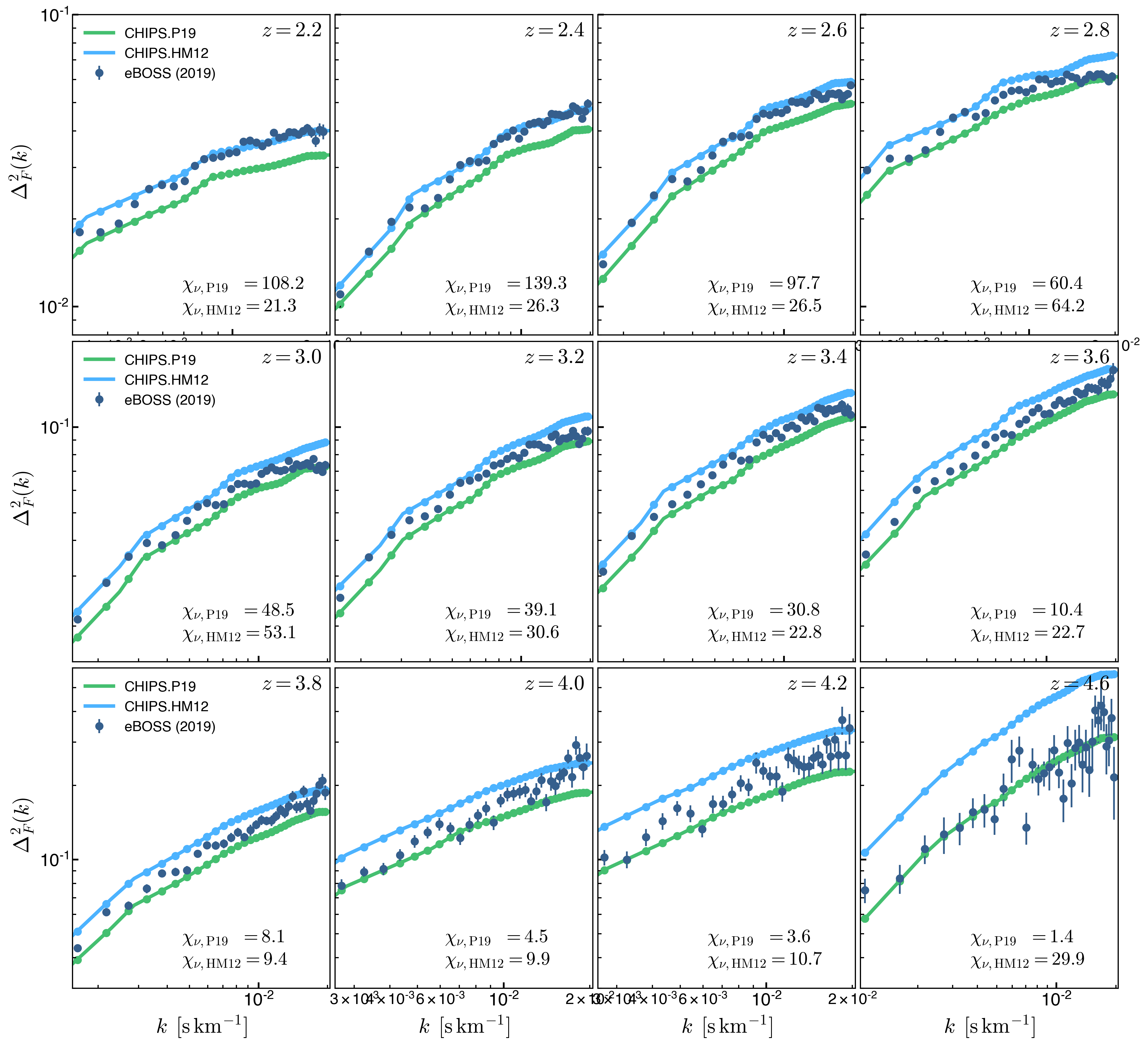
Now comparing in the $k \leq 0.01 \, \mathrm{s} \, \mathrm{km}^{-1}$ range:

For the large scale comparison with the eBOSS data the differences are much larger

\