Comparison to Ewald Simulation (Complete)
Cholla Simulations:
Box Size = 50 Mpc/h
Numerical Size: Uniform Grid \(2048^3\) cells, and \(2048^3\) dark matter particles
SPH Simulations:
Box Size = 10 Mpc/h
Numerical Size: \(512^3\) gas particles, and \(512^3\) dark matter particles
Interpolation to the Grid
To interpolate the particle data obto the grid, I use the kernel function used in Gadget2. The kernel as a function of distance \(r\) and smoothing length \(h\) is given by:
\[W(r, h)=\frac{8}{\pi h^{3}}\left\{\begin{array}{ll} 1-6\left(\frac{r}{h}\right)^{2}+6\left(\frac{r}{h}\right)^{3}, & 0 \leqslant \frac{r}{h} \leqslant \frac{1}{2} \\ 2\left(1-\frac{r}{h}\right)^{3}, & \frac{1}{2}<\frac{r}{h} \leqslant 1 \\ 0, & \frac{r}{h}>1 \end{array}\right.\]The interpolation is done as following:
\[\rho(x)=\sum_{j=1}^{N} m_{j} W\left(\left|\mathbf{r}\right|, h_{i}\right)\] \[\rho_{\mathrm{HI}}(x)=\sum_{j=1}^{N} m_{\mathrm{HI},j} W\left(\left|\mathbf{r}\right|, h_{i}\right)\] \[v(x)= \frac{\sum_{j=1}^{N} \rho_{j} v_j W\left(\left|\mathbf{r}\right|, h_{i}\right)}{ \sum_{j=1}^{N} \rho_{j} W\left(\left|\mathbf{r}\right|, h_{i}\right)}\]I interpolate the particle data onto a grid ( \(512^3\) cells ). For the interpolation I used two different methods:
Gather 64: Measure the distance that encloses 64 neighboring particles and use that distance as the smoothing length when computing the kernel weights.
Scatter: Use the smoothing lengths of the neighboring particles when computing the kernel weights.
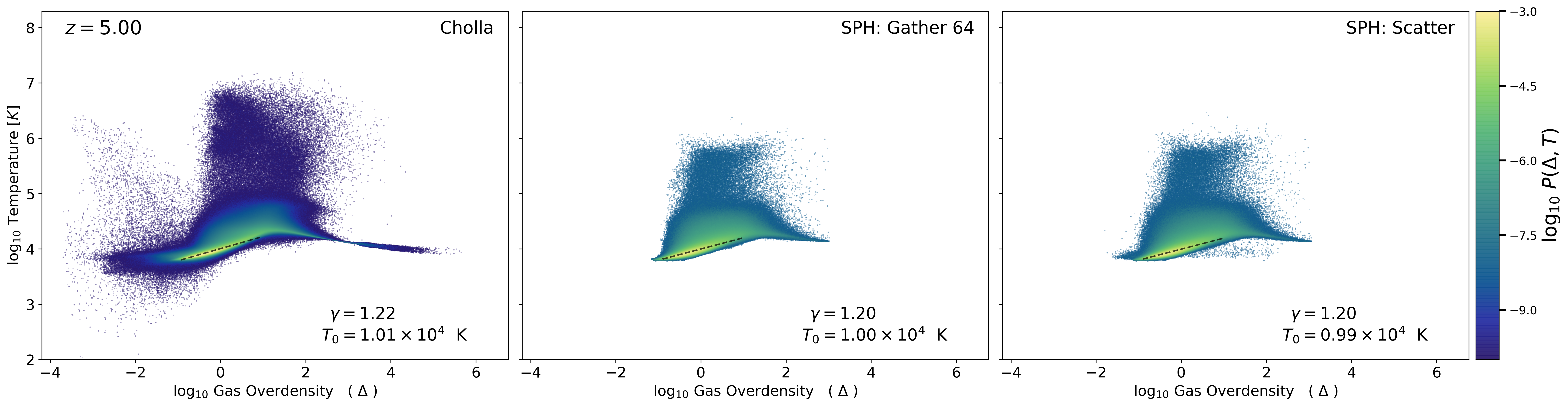
Phase Diagram Comparison
After interpolating the particle data into a uniform grid, I measure the volume weighted temperature-density distribution for the two snapshots and compare to the ones from the Cholla Simulation:
z = 5
z= 5.5
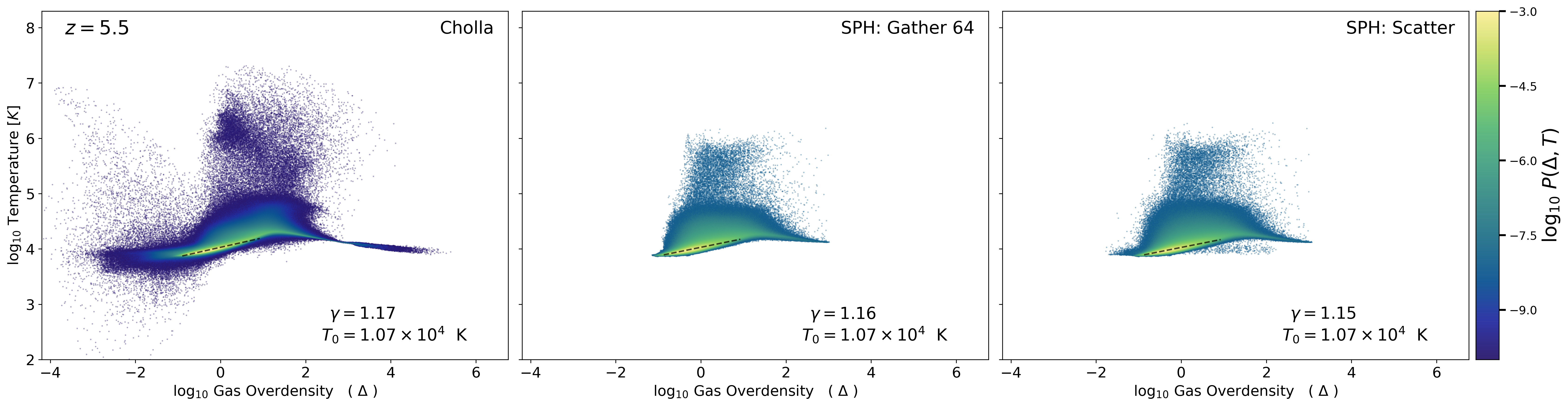
Both simulations have almost identical power law temperature-density relations.
Density Distribution Comparison
Next I measured the gas density and the neutral hydrogen density distributions on the Grid-SPH data and compared to the ones in the Cholla simulation ( only for z=5):
Left Panel: Gas density distribution.
Center Panel: HI density distribution.
Right Panel: Neutral fraction distribution.
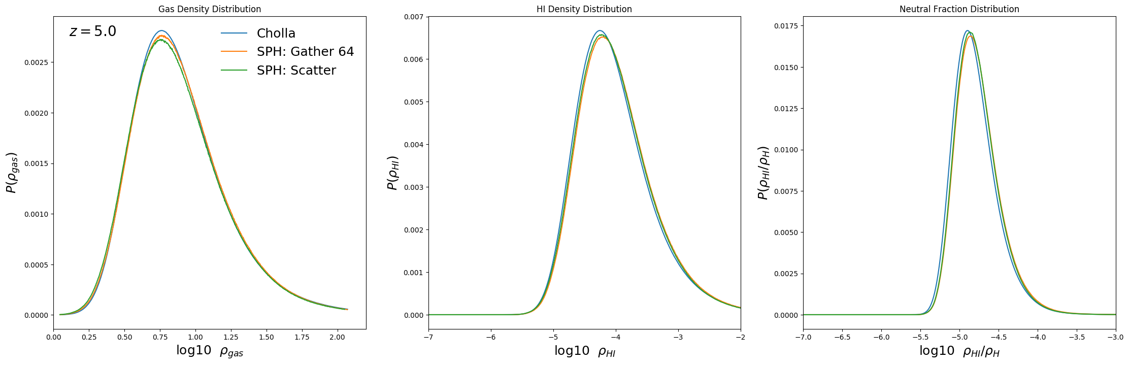
The density distributions for both simulations are surprisingly similar.
Transmitted Flux Calculation:
The following figure shows the Optical Depth \(\tau\) and transmitted flux \(F\) for a single skewer from the Cholla simulation at z=5:
![]()
The optical depth \(\tau\) is computed from the integral of a Gaussian profile for each absorber, this is given by:
\[\tau_{j} = \frac{\pi e^{2} \lambda_0 f_{12}}{m_{e} c H} \sum_i n_{\mathrm{HI},i} \frac{ erf(y_{j+1/2,i}) - erf(y_{j-1/2,i}) }{2}\] \[y_{j+1/2,i} = ( v_{j+1/2} - v_{\mathrm{H},i} - v_{\mathrm{LOS},i} )/b_i\] \[y_{j-1/2,i} = ( v_{j-1/2} - v_{\mathrm{H},i} - v_{\mathrm{LOS},i} )/b_i\]View appendix at the end for a discussion about using a Voigt profile instead of a Gaussian profile
Effective Optical Depth:
After computing the transmitted flux \(F\) for 16384 skewers I compute the effective optical depth \(\tau_{eff} = - \mathrm{ln}\, \langle F \rangle\). The following figure shows the evolution of \(\tau_{eff}\) as a function of redshift for the Cholla simulation, additionally I show \(\tau_{eff}\) computed from the same number of skewers crossing the SPH(Grid) box for the two snapshots I have.
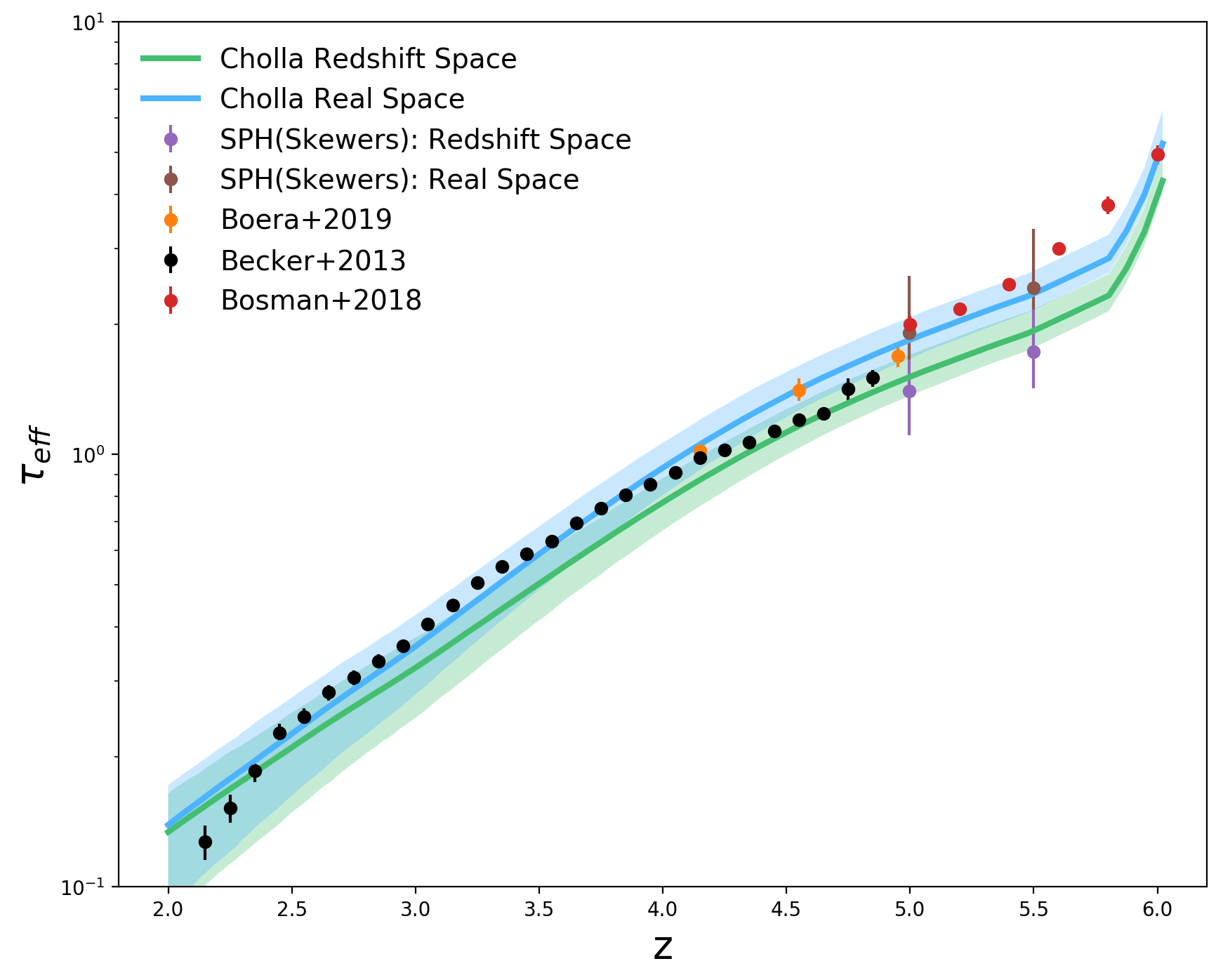
The measurements I get from the SPH simulation are consistent with the Cholla simulation, in redshift space the SPH \(\tau_{eff}\) is somewhat lower to the Cholla measurement, but in real space \(\tau_{eff}\) is very similar in both simulations and also consistent with the values reported on Puchwein et al. 2019.
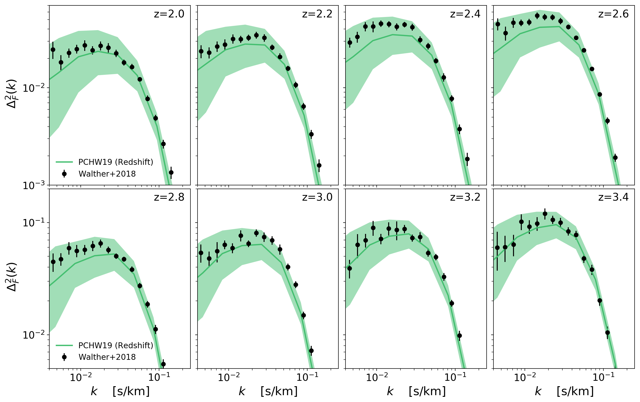
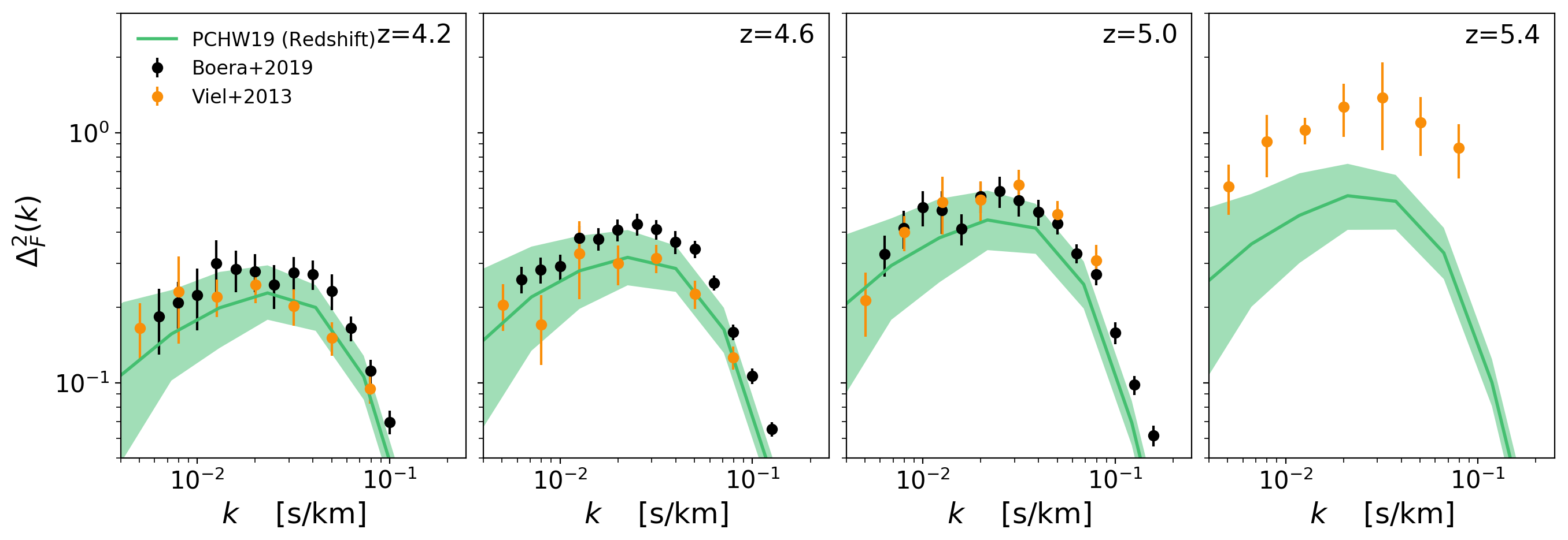
Transmitted Flux Power Spectrum
This is the Transmitted Flux Power Spectrum measured in Redshift space:
Appendix: Voigt Profile
From Puchwein et al. 2015: Here
Synthetic Lyman α forest spectra:
We compute synthetic Lyman \(\alpha\) forest spectra in post-processing. This allows us to directly compare the effective optical depth for absorption as well as other statistics of the simulated spectra to observations. We select 5000 randomly placed lines of sight through each output of the simulation box, along directions parallel to one of the coordinate axes (randomly selected among x, y and z). Each line of sight is represented by 2048 pixels. We then compute the neutral hydrogen density, temperature and velocity of the IGM along these lines of sight by adding up the density contributions and averaging the temperatures and velocities of all SPH particles whose smoothing lengths are intersected. Our calculation of the spectra accounts for Doppler shifts due to bulk flows of the gas as well as for thermal broadening of the Lyman \(\alpha\) line (see e.g. Bolton & Haehnelt 2007). This yields the optical depth, \(\tau\) , for Lyman \(\alpha\) absorption as a function of velocity offset along each line of sight, which can then be easily converted into a transmitted flux fraction, \(F = e^{ −τ}\) , as a function of wavelength or redshift. *
From Bolton & Haehnelt 2007: Here
We construct synthetic spectra from the output of the radiative trans- fer simulations as follows. Each line-of-sight is rebinned to have N = 4096 pixels of proper width \(\delta R\), each of which has a neutral hydrogen number density \(n_{\mathrm{HI}}\) , temperature \(T\), peculiar velocity \(v_{\mathrm{pec}}\) and Hubble velocity \(v_{\mathrm{H}}\) associated with it. The Lya optical depth in each pixel is computed assuming a Voigt line profile, such that the optical depth in pixel \(i\) corresponding to Hubble velocity \(v_{\mathrm{H}}(i)\) is:
\[\tau_{\alpha}(i)=\frac{c \sigma_{\alpha} \delta R}{\pi^{1 / 2}} \sum_{j=1}^{N} \frac{n_{\mathrm{HI}}(j)}{b(j)} H(a, x)\]Here \(b=\left(2 k_{\mathrm{B}} T / m_{\mathrm{H}}\right)^{1 / 2}\) is the Doppler parameter, \(\sigma_{\alphaα} = 4.48 \times 10^{−18} \mathrm{cm}^2\) is the Lya scattering cross-section and \(H(a, x)\) is the Hjerting function (Hjerting 1938)
\[H(a, x)=\frac{a}{\pi} \int_{-\infty}^{\infty} \frac{\mathrm{e}^{-y^{2}}}{a^{2}+(x-y)^{2}} \mathrm{d} y,\]where \(x=\left[v_{\mathrm{H}}(i)-u(j)\right] / b(j)\) , \(u(j)=v_{\mathrm{H}}(j)+v_{\mathrm{pec}}(j)\), \(a = \Lambda_{\alpha} \lambda_{\alpha} / 4 \pi b(j)\) , \(\Lambda_{\alpha}=6.265 \times 10^{8} \mathrm{s}^{-1}\) is the damping constant and \(\lambda_{\alpha}=1215.67 \AA\) is the wavelength of the Lyα transition.
I computed the optical depth using the Voigt profile described above to the Gaussian profile and the differences where less than 1%. I only did this for a single skewer because the computational cost of using the Voigt profile is much larger.