Effective Optical Depth from Density Distributions
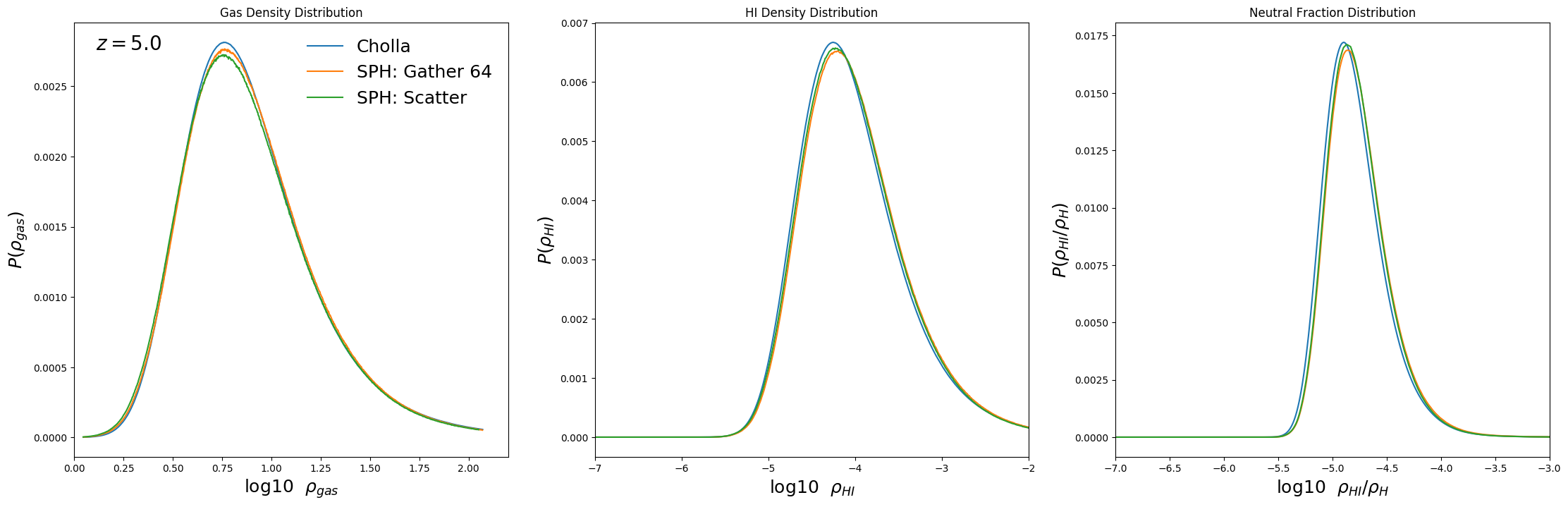
From the volume weighted density distributions below it’s possible to compute an approximate value for the effective optical depth in the simulations
From Bolton et al. 2009
Assuming the IGM is highly ionised and in photoionisation equilibrium with the metagalactic UV background, and the low density IGM \((\Delta = \rho/ \langle \rho \rangle \leq 10)\) follows a power-law temperature density relation, \(T = T_0 \Delta^{\gamma -1}\) (Hui & Gnedin 1997; Valageas et al. 2002), the Lyα optical depth at z >∼2 may be written as:
\[\begin{aligned} \tau \simeq & 1.0 \frac{\left(1+\chi_{\mathrm{He}}\right)}{\Gamma_{-12}}\left(\frac{T_{0}}{10^{4} \mathrm{K}}\right)^{-0.7}\left(\frac{\Omega_{\mathrm{b}} h^{2}}{0.024}\right)^{2}\left(\frac{\Omega_{\mathrm{m}} h^{2}}{0.135}\right)^{-1 / 2} \left(\frac{1+z}{4}\right)^{9 / 2} \Delta^{2-0.7(\gamma-1)} \end{aligned}\]where \(\Omega_b\) and \(\Omega_m\) are the present day baryon and matter densities as a fraction of the critical density, \(h = H_0/100 \,\,\mathrm{km} \mathrm{s}^{−1} \mathrm{Mpc}^{−1}\) for the present day Hubble constant \(H_0\), \(\Delta = \rho/ \langle \rho \rangle\) is the normalised gas density, \(T_0\) is the gas temperature at mean density, \(\gamma\) is the slope of the temperature density relation and \(\Gamma_{−12} = \Gamma_{HI}/10^{−12} \mathrm{s}^{−1}\) is the hydrogen photo-ionisation rate. The power-law temperature dependence is due to the case-A HII recombination coefficient, and \(\chi_{\mathrm{He}}\) accounts for the extra electrons liberated during HeII reionisation; \(\chi_{\mathrm{He}} = 1.08\) prior to HeII reionisation and \(\chi_{\mathrm{He}} = 1.16\) afterwards for a helium fraction by mass of \(Y = 0.24\) (Olive & Skillman 2004).
The effective optical depth can then be estimated by integrating over all possible IGM densities \(\Delta\):
\[e^{-\tau_{\mathrm{eff}}}=\int_{0}^{\infty} d \Delta P_{V}(\Delta) \int d T P(T | \Delta) e^{-\tau(T, \Delta)}\]Again, we emphasise that this ignores peculiar velocities of the gas, line blending (and indeed the wings of every line), and the clustering of the absorbers, but it provides a qualitative description of the evolving transmission.
An alterenative Calculation:
Following the previous method I think I could use the HI distribution directly from the simulation, so instead of \(\Delta\) I could use \(\Delta_{\mathrm{HI}} = \rho_{\mathrm{HI}} / \langle \rho_{\mathrm{HI}} \rangle\), leading to:
\[e^{-\tau_{\mathrm{eff}}}=\int_{0}^{\infty} d \Delta_{\mathrm{HI}} P_{V}(\Delta_{\mathrm{HI}}) \int d T P(T | \Delta_{\mathrm{HI}}) e^{-\tau(T, \Delta_{\mathrm{HI}})}\]and the optical depth for each element can be computed as the amplitude of the absorption line:
\[\tau=\frac{\pi e^{2} \lambda_0}{m_{e} c H} \frac{f_{12}}{\sqrt{\pi}} \frac{n_{\mathrm{HI}}}{b}\]